UNDER CONSTRUCTION

In this post, we will consider various methods of sampling. We will go (roughly) in order of preference of methods. Ideally, we can invert the CDF for our distribution for sampling, but this isn’t always possible. We present our methods in increasing order of desperation overall, however we note that importance sampling is rather a solution to the problems presented by rejection sampling, and Gibbs sampling is a special case of Metropolis. Some of the later topics on Metropolis/Gibbs were faciliated by fruitful conversations with Michael Lewis.

Inverse Sampling
Rejection Sampling
Importance Sampling
Metropolois Hastings
Gibbs Sampling

Inverse Sampling

We will present a slightly more general treatment here than is usually seen. Imagine that we wish to sample from some probability measure $\nu$ but only have access to a probability distribution $\mu$ (eg. $\mu = \textrm{Unif}[0,1]$, a random number generator). Now if we can generate samples from $\mu$, is there a way to obtain samples from $\nu$? We could if there was some sort of map which took elements of the $\sigma$-algebra of $\mu$ to $\nu$.

Given i.i.d samples $\{x_i\}$ sampled from $\mu$, how do we generate samples from $\nu$. The solution lies in the push forward map or an transport map. More precisely, we say

\[T \# \mu = \nu\]

\[\nu(A) = \mu(T^{-1}(A)).\]

In the case of one dimension, it turns out there is only one such map. Let $F_{\nu}$ and $F_{\mu}$ be defined by

\[F_{\nu}(x) = \int_{-\infty}^x d\nu(x)\] \[F_{\mu}(x) = \int_{-\infty}^x d\mu(x).\]

Then the unique map which satisfies $T \# \mu = \nu$ is

\[T = F_{\nu}^{-1} \circ F_{\mu}.\]

Such a map always exists even in higher dimensions, assuming that $\mu << \mathcal{L}$. This is a result by [Brenier, 95]. In fact, he showed that

\[T(x) = \nabla \Psi(x),\]

where $x \mapsto \Psi(x)$ is a strictly convex function. Moreover $x \mapsto T(x)$ minimizes the so called Wasserstein distance:

\[\mathcal{W}(\mu,\nu) = \inf_{T \# \mu = \nu} \int \left | x - T(x)\right|^2 d\mu(x).\]

Counterexample:

It’s easy to see that such a map does not always exist, even in one dimension. Take as a counterexample, $\mu = \delta_{x=0.5}$ and $\nu = \frac{1}{2}\delta_{x=0}+\frac{1}{2}\delta_{x=1}$. This of course doesn’t make sense as a function, since the mass needs to split itself across $x=0$ and $x=1$. The same would hold if $\nu = \textrm{Unif}[0,1]$ in fact. So the essential rule to remember is mass can’t split.

Now that we’ve reviewed some Optimal Transport Theory (see Cedric Villani’s excellent books on the topic if you’re interested), let’s get back to the main point. Now that we know that $T$ transports the mass of $\mu$ to $\nu$, let’s use it to sample $\nu$ from $\mu$. We will focus on one dimension now.

Example 1: Sampling Binomial from Uniform

We know that if $x \sim \textrm{Unif}[0,1]$ then $\Phi^{-1}(x) \sim \textrm{Bin}(n,p)(k).$ First define the CDF of the binomial distribution:

\[\Phi(k) = \sum_{j \leq k} {n \choose j} p^j (1-p)^{n-j}.\]

Thus $\Phi^{-1}(x) = \min_{k} \{ \Phi(k) \geq x\}.$

Thus for any $x$ sampled from $[0,1]$, we just find the corresponding minimum value of $k$ such that $\Phi(k) \geq x$.

s = np.random.uniform(0,1,1000)
plt.hist(s)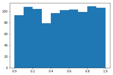

import math
def nCr(n,r):
    f = math.factorial
    return f(n) / f(r) / f(n-r)
def binomial(n,p,k):
    return nCr(n,k)*(p**k)*(1-p)**(n-k)
def binomial_cdf(n,p,k):
    return sum([binomial(n,p,j) for j in range(0,k)])
def binomial_sample(n,p,x):
    for j in range(0,n):
        if binomial_cdf(n,p,j)> x:
            return j-1
    
p = 0.5
n = 100

Now let’s plot the results

binom_samp=[binomial_sample(n,p,x) for x in s]
plt.hist(binom_samp)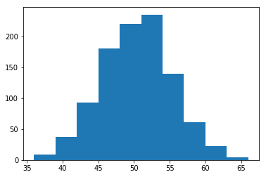

Example 2: Sampling binomial from normal

s = np.random.normal(0,1,1000)
phi_mu = [0.5 + 0.5*math.erf(x) for x in s]
T = [binomial_sample(n,p,x) for x in phi_mu]
plt.hist(T)

Rejection Sampling

Obtain a sample ${\displaystyle y}$ from distribution ${\displaystyle Y}$ and a sample ${\displaystyle u}$ from ${\displaystyle \mathrm {Unif} (0,1)}$ (the uniform distribution over the unit interval).
Check whether or not ${\textstyle u<f(y)/Mg(y)}$
If this holds, accept ${\displaystyle y}$ as a sample drawn from ${\displaystyle f}$;
if not, reject the value of ${\displaystyle y}$ and return to the sampling step.

The algorithm will take an average of ${\displaystyle M}$ iterations to obtain a sample.

Example:

Let $f(x) = 1_{x>5}(x) \frac{1}{\sqrt{2\pi}} e^{-x^2/2}.$ Then choose $g(x) = \frac{1}{\sqrt{2\pi}} e^{-x^2/2}.$

Then $f \leq g$ with constant $M=1$.

def rejection_sample(cutoff):
    g = np.random.normal(0,1,10000)
    f = [x for x in g if x > cutoff ]
    P_sim = len(f)/len(g)
    return P_sim

Now let’s see how well this does. We’ll do that by evaluating the actual area under the Gaussian for $x > \textrm{cutoff}$. First let’s define some important functions:

def phi(x):
    'Cumulative distribution function for the standard normal distribution'
    return (1.0 + math.erf(x / np.sqrt(2.0))) / 2.0
def actual_value(cutoff):
    return 1 - phi(cutoff)

rs_estimates = []
actual_values = []
for k in range(1,4):
    rs_estimates.append(rejection_sample(k))
    actual_values.append(actual_value(k))
plt.plot(rs_estimates,label='RS')
plt.plot(actual_values,label='Actual')
plt.legend()

Metropolis Hastings Algorithm

Let’s assume we can sample from some distribution $q(x)$ and we wish to sample from a known distribution $p(x)$.

Our goal is to construct a Markov Chain $Q$ whose stationary distribution is $p(x)$. This would mean that

\[\pi(x') Q(x \lvert x')A(x \lvert x') = Q(x' \lvert x) \pi(x) A (x' \lvert x),\]

for $\pi(x) = p(x)$ where $Q$ is the transition matrix and $A$ is the acceptance probability. The above is known as a detailed balance. In other words, the flow of mass $x \mapsto x'$ is the same as $x' \mapsto x$. Our acceptance probability is therefore

\[\frac{A(x' \lvert x)}{A(x \lvert x')} = \frac{Q(x \lvert x') p(x')}{Q(x' \lvert x) p(x)}=: H(x'|x) .\]

We want to sample $x'$ from $Q(\cdot \lvert x)$ and accept it with probability $A(x' \lvert x)$.

What remains is:

What Q do we choose? If we could sample from $p$ directly, we could just choose $Q = p$ with $A = 1$ and we would be done. But generally we can’t, so we try to find something which is “close” to the distribton p in some sense.
What A do we choose? We want the probability of acceptance to be high, but any choice of $A$ satisfying the above equation will work. Note that if $T$ is close to $p$ then $A \sim 1$.

A common choice of $A$ is

\[A(x' \lvert x) = \min \left( 1, \frac{Q(x \lvert x') p(x')}{Q(x' \lvert x) p(x)} \right) = \min \left(1, H(x' \lvert x)\right).\]

Proof of balance: Note that $H(x'\lvert x) H(x \lvert x') = 1$.

Case 1: $H(x' \lvert x) = 1$. Then $A(x' \lvert x) = A(x \lvert x') = 1$
Case 2: $H(x' \lvert x) > 1$. Then $A(x' \lvert x) = 1$. Since $H(x \lvert x') < 1$ by the above, we have $A(x \lvert x') = \frac{Q(x' \lvert x) p(x)}{Q(x \lvert x') p(x')}$ which balances the above.
Case 3: $H(x' \lvert x) < 1$. Then $A(x \lvert x') = 1$

The algorithm is defined as follows:

Algorithm

1) Sample $x_t \sim q(x \lvert x_{t-1})$.

2) Define

\[\alpha = \min\left\{1,\frac{q(x_t \lvert x_{t-1}) p(x_{t-1})}{q(x_{t-1} \lvert x_t) p(x_t)} \right\}.\]

3) Sample $u \sim \textrm{Unif}[0,1]$.

If $u < \alpha$, then accept and return $x_t$.
Otherwise set $x_t = x_{t-1}$.

4) Repeat step 1).

Example:

def p(x):
    return (1/np.sqrt(2*np.pi))*np.exp(-(x**2)/2)


def T(xprime,x,delta=0.1):
    if np.abs(xprime-x) < delta:
        return 1
    else:
        return 0

def A(xprime,x,delta=0.1):
    alpha = min(1, (p(xprime))/p(x))
    u = np.random.uniform(0,1)
    if u < alpha:
        return 1
    else:
        return 0

def metropolis(max_iterations=100000,delta=0.1):
    x_next = 0
    x_vals=[]
    for n in range(max_iterations):
        x_candidate = np.random.uniform(x_next-delta,x_next+delta)
        
        accept = A(x_candidate,x_next)
        if accept == 1:
            x_next = x_candidate
        else:
            x_next = x_next
        x_vals.append(x_next)
    return x_vals

x_vals = metropolis()

Gibbs Sampling

Note that the MH algorithm treats $p(x)$ as a black box and does not leverage any particular structure of $p(x)$. Similarly, the proposal distribution we choose typically does not depend on p(x) and also does not leverage any structure of $p(x)$.

Gibbs sampling is a MCMC algorithm that repeatedly samples from the conditional distribution of one variable of the target distribution p, given all of the other variables. Gibbs sampling works as follows:

Imagine that we have $K$ variables $\mathbf X = (x_1,x_2,\cdots,x_k)$ and we can calculate the posterior conditional distributions exactly. As before, let’s try to sample from $P(\mathbf X \lvert D)$ by constructing a Markov Chain.

In this case, we will choose $i$ randomly from $\{1,2,\cdots,K\}$ and hold all variables not equal to $i$ fixed to their previous values. We denote this vector as $x_{-i}$. Then we wish to sample a new value of $x_i$ from $p(x_i' \lvert x_{-1})$.

\[\alpha = \frac{ T(x_i',x_{-i} \lvert x_i, x_{i-1}) p(x_i,x_{i-1})}{T(x_i,x_{-i} \lvert x_i', x_{i-1}) p(x_i' ,x_{i-1})}.\]

Since we can compute the posteriors directly, we set

\[T(x_i', x_{-i} \lvert x_i, x_{i-1}) = \frac{1}{K} p(x_i' \lvert x_{i-1}).\]

Then $\alpha = \frac{ p(x_i' \lvert x_{i-1}) p(x_i \lvert x_{i-1})p(x_{i-1})}{p(x_i \lvert x_{i-1}) p(x_i' \lvert x_{i-1})p(x_i' \lvert x_{-1}} = 1,$

so we always accept the candidate sample in Gibbs sampling.

Dorian Goldman

Monte Carlo Sampling Methods