Markov Decision Processes
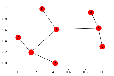
In this post, we will explore (literally!) how to find an optimal sequence of actions to reach a desired goal. These are the basic principles upon which Alpha Go was built (but in a much simpler setting). Before we get into the details, let’s construct a basic graph. Our goal will be to go from 0 to 7 in this example.
import networkx as nx
points_list = [(0,1), (1,5), (5,6), (5,4), (1,2), (2,3), (2,7)]
G=nx.Graph()
G.add_edges_from(points_list)
pos = nx.spring_layout(G)
nx.draw_networkx_nodes(G,pos)
nx.draw_networkx_edges(G,pos)
nx.draw_networkx_labels(G,pos)
plt.show()
Our goal is to find a sequence of actions, denote by policty \(\pi\) to maximize the total reward: \(\mathbb{E}[R \lvert \pi] = \int p(\tau \lvert \pi) R(\tau)\) where \(\tau\) is the space of all paths, ie \(\tau = (a_0,s_0,r_0,a_1,s_1,r_1,\cdots,a_t,s_t,r_t)\).
What is the reward?
We will define this below in such a way as to take advantage of our goal and the structure of the graph. This is a common thing to do in reinforcement learning.
From the Markov property we have \(p(\tau \lvert \pi) = \prod_{t=1}^{T-1} p(s_{t+1}\lvert s_t,a_t) \pi (a_t \lvert s_t).\)
We will assume that \(\pi(a_t \lvert s_t)\) is some stochastic policy, which has a form of
\[\pi (a_t \lvert s_t) = \frac{e^{-\theta_{s_t,s_{t-1}}}}{\sum_k e^{-\theta_{s_t,s_k}}}\]The policy gradient trick:
Observe that \(\begin{align} \nabla_{\theta} \mathbb{E}[R \lvert \pi] &= \int \nabla_{\theta} p (\tau \lvert \pi) R(\tau) \\ &= \int \frac{\nabla_{\theta} p(\tau \lvert \pi)}{p(\tau \lvert \pi)} p(\tau \lvert \pi) R(\tau)\\ &= \mathbb{E}_p\left[ \nabla_{\theta} \log p(\tau \lvert \pi) R(\tau)\right] \end{align}\)
In other words, we can write this as an expectation once again, and therefore use samples from our data! But even more importantly:
\[\begin{align} \log p(\tau \lvert \pi) &= \log \prod_{t=1}^{T-1} p(s_{t+1}\lvert s_t,a_t) \pi (a_t \lvert s_t)\\ &=\sum_{t=1}^{T-1} \log p(s_{t+1} \lvert s_t,a_t) + \sum \log \pi(a_t \lvert s_t) \end{align}\]The amazing thing here is that while our policy depends on our choice of \(\theta_{s_{t},s_{t-1}}\), \(p(s_{t+1} \lvert s_t,a_t)\) does not!
Our setting
In our case, we have 7 nodes labeled \(k=0,1,\cdots,7\) and we make the softmax prior:
\(\pi (k \lvert m ) = \frac{e^{-\theta_{k,m}}}{\sum_k e^{-\theta_{k,m}}},\) which is the transition probability of going from node m to node k. How do we define the rewards?
Choice of Reward:
- We want to have a negative reward when we hit a barrier - ie. there is no edge in the graph. We set the reward in this case to be \(-1\).
- We want to favor possible directions (even if they haven’t lead to the reward yet). So we set the reward to be \(1\) if the edge exists.
- We define a reward of \(100\) if our path reaches the goal: node 7.
# how many points in graph? x points
MATRIX_SIZE = 8

# create matrix x*y
R = np.matrix(np.ones(shape=(MATRIX_SIZE, MATRIX_SIZE)))
R *= -1

# assign zeros to paths and 100 to goal-reaching point
for point in points_list:
    print(point)
    if point[1] == goal:
        R[point] = 100
    else:
        R[point] = 0

    if point[0] == goal:
        R[point[::-1]] = 100
    else:
        # reverse of point
        R[point[::-1]]= 0

# add goal point round trip
R[goal,goal]= 100

R
Output:
(0, 1)
(1, 2)
(2, 7)
matrix([[  -1.,    0.,   -1.,   -1.,   -1.,   -1.,   -1.,   -1.],
        [   0.,   -1.,    0.,   -1.,   -1.,   -1.,   -1.,   -1.],
        [  -1.,    0.,   -1.,   -1.,   -1.,   -1.,   -1.,  100.],
        [  -1.,   -1.,   -1.,   -1.,   -1.,   -1.,   -1.,   -1.],
        [  -1.,   -1.,   -1.,   -1.,   -1.,   -1.,   -1.,   -1.],
        [  -1.,   -1.,   -1.,   -1.,   -1.,   -1.,   -1.,   -1.],
        [  -1.,   -1.,   -1.,   -1.,   -1.,   -1.,   -1.,   -1.],
        [  -1.,   -1.,    0.,   -1.,   -1.,   -1.,   -1.,  100.]]
Step 1: Initializiation
We assume that we can go in any direction, so we assume that \(\theta_{km} \equiv 0\), giving equal probability to each direction.
# Initialize Weights
theta = np.matrix(np.zeros(shape=(8,8)))
theta
Output:
matrix([[ 0.,  0.,  0.,  0.,  0.,  0.,  0.,  0.],
        [ 0.,  0.,  0.,  0.,  0.,  0.,  0.,  0.],
        [ 0.,  0.,  0.,  0.,  0.,  0.,  0.,  0.],
        [ 0.,  0.,  0.,  0.,  0.,  0.,  0.,  0.],
        [ 0.,  0.,  0.,  0.,  0.,  0.,  0.,  0.],
        [ 0.,  0.,  0.,  0.,  0.,  0.,  0.,  0.],
        [ 0.,  0.,  0.,  0.,  0.,  0.,  0.,  0.],
        [ 0.,  0.,  0.,  0.,  0.,  0.,  0.,  0.]])
We define the corresponding probabilites based on \(\theta\), which, as expected are uniform across possible paths
# Initialize Weights to be learned
for k in range(8):
    W[k]=softmax(theta[k].squeeze())
W
Output:
matrix([[ 0.125,  0.125,  0.125,  0.125,  0.125,  0.125,  0.125,  0.125],
        [ 0.125,  0.125,  0.125,  0.125,  0.125,  0.125,  0.125,  0.125],
        [ 0.125,  0.125,  0.125,  0.125,  0.125,  0.125,  0.125,  0.125],
        [ 0.125,  0.125,  0.125,  0.125,  0.125,  0.125,  0.125,  0.125],
        [ 0.125,  0.125,  0.125,  0.125,  0.125,  0.125,  0.125,  0.125],
        [ 0.125,  0.125,  0.125,  0.125,  0.125,  0.125,  0.125,  0.125],
        [ 0.125,  0.125,  0.125,  0.125,  0.125,  0.125,  0.125,  0.125],
        [ 0.125,  0.125,  0.125,  0.125,  0.125,  0.125,  0.125,  0.125]])
Step 2: Choose a stochastic policy
In our setting if are at node $k(t)$ at time t, then \(a_{k(t)} \sim \textrm{Mult}\left(\pi_{0k},\cdots,\pi_{7k}\right)\) We do this in Python via:
s_next = np.where(np.random.multinomial(1, np.array(W[s_current,:]).squeeze(), size=1)==1)[1][0]Step 2: Oberve reward and update parameters in good directions
Thus we want to find the best path. At each observation we want to gradient descent in the direction of best gradient:
\[\theta_{km}^t= \theta_{km}^{t-1} - R(t) \nabla_{\theta} \log \pi (k \lvert m)\]For this we do a simple computation:
\[\log \pi (k \lvert m) = - \theta_{km} - \log \left( \sum_l e^{-\theta_{lm}}\right).\]Thus
\[\nabla_{\theta_{km}} \log \pi (k \lvert m) = \pi(k \lvert m) - 1,\]a relative simple equation!
We implement it as gradient below:
def gradient(k,m,alpha=0.1):
    #denom = sum([np.exp(-theta[k,l]) for l in range(8)])
    return R[k,m]*(W[k,m]-1)
And the softmax function:
def softmax(t):
    return np.exp(-t)/np.sum(np.exp(-t))
We see here that we want to nudge the parameters in the good directions - ie. the one with highest payoffs. This is very analogous to importance sampling
Step 3: Keep on iterating and learning
We now show the full code below which initializes uniform weights then does 100 iterations of exploring the graph. The shortest path is then recorded as the “best” path and plotted below.
s_current = 0
# Initialize Weights
W = np.matrix(np.ones(shape=(8,8)))
#W *= 1/8
# Initialize Weights
theta = np.matrix(np.zeros(shape=(8,8)))
# Initialize Weights to be learned
for k in range(8):
W[k]=softmax(theta[k].squeeze())
best_path=[]
best_length=1000
found_after = 0
for simulation in range(100):
s_current = 0
# Initialize Weights
theta = np.matrix(np.zeros(shape=(8,8)))
# Initialize Weights to be learned
for k in range(8):
W[k]=softmax(theta[k].squeeze())
path=[]
for t in range(10):
reward=-1
while reward < 0:
s_next = np.where(np.random.multinomial(1, np.array(W[s_current,:]).squeeze(), size=1)==1)[1][0]
reward = R[s_current,s_next]
path.append((s_current,s_next))
if reward == 100:
if len(path) < best_length:
best_path = path
best_length=len(best_path)
found_after = simulation
break
#print (s_current,s_next,R[s_current,s_next])
reward_next = R[s_current,s_next]
#print (s_next)
for m in range(8):
theta[s_current,m] = theta[s_current,m] + gradient(s_current,m,alpha=0.01)
for k in range(8):
W[k]=softmax(theta[k].squeeze())
s_current = s_next
print ("Found best path " + str(best_path) + " after " + str(found_after) + " simulations")
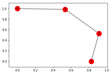
# map cell to cell, add circular cell to goal point
points_list = best_path
goal = 7
G=nx.Graph()
G.add_edges_from(points_list)
pos = nx.spring_layout(G)
nx.draw_networkx_nodes(G,pos)
nx.draw_networkx_edges(G,pos)
nx.draw_networkx_labels(G,pos)
plt.show()Output:
Found best path [(0, 1), (1, 2), (2, 7)] after 5 simulations