We will go over two main methods in this post - Random Forests and Gradient Boosting, falling under the categories of Bagging and Boosting methods respectively. Bagging methods take multiple trees or weak learners, trained in parallel, then combine the results. While boosting iterates and corrects the errors on the residuals in a recursive manner.
They both have their benefits and drawbacks - here is a quick summary of some of them.
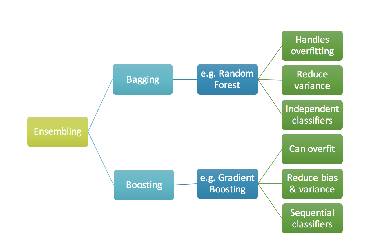
Question: Which one should you use?
For a nice comparison, see https://github.com/zygmuntz/misc/tree/master/gbm_vs_rf. Essentially it appears that Gradient Boosted Trees have replaced Random Forests as the method of choice on Kaggle problems, and seem to provide overall better performance in a widge range of scenarios. However they are not easily parallelized (can you think of why before reading this post?) and thus take much longer to train. As with any modeling decision, one must consider what is the most important - model performance, training time, prediction time, or some combination of the above.
Random Forests
Random Forests are a simple but powerful extension of decision trees which help to prevent overfitting. If you haven’t read my post on Decision Trees, please read that one first. Once you understand how decision trees work, building a random forest is an easy extension. One simply chooses random subsets of \(\tilde K < K\) features where \(K\) is the number of features and \(J\) random rows. You then you train \(T\) decision trees and average the results over the trees (you can also take the mode or median if you wish). To do variable importance you simply average out over all of the trees as well.
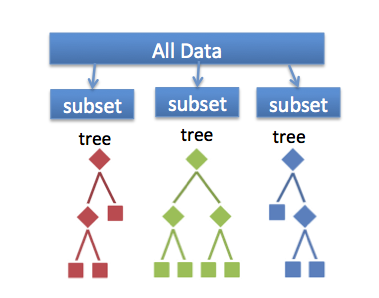
In other words, our prediction would be
\[\hat p_{RF}(y | x) = \frac{1}{K} \sum_{k=1}^K \hat p_K (y \vert x),\]where \(\hat p_K\) is the estimator for an individual tree and \(\hat p_{RF}\) is the estimator for the final tree based on averaging over the decision trees. Note that we can also take the mode or median instead of the average here.
The main advantages of Random Forests are:
- Not prone to over fitting due to the averaging of many trees.
- Easy to implement ‘off the shelf’.
- Easy to parallelize since the decision trees do not need to exchange information when being constructed.
Gradient Boosting
The main idea in gradient boosting is to leverage the pattern in residuals and strenghten a weak prediction model, until our residuals become randomly (maybe random normal too) distributed.
Continous case
There is a lot of confusing notation and discussion around gradient boosting, when ultimately it is just the gradient flow in a functional space (ie. \(L^2\)).
Imagine that we have a loss funciton \(\mathcal{L}:X \times Y \to \mathbb{R}\) equipped with some joint probability distribution \(p(y,x)\) such that \(\mathcal{L} \in L^p(dp)\). For example, in the ordinary least squares setting, we would seek to find \(f\) such that
\[f = \textrm{argmin}_f \mathbb{E}_{x,y} \frac{1}{2} (y - f(x))^2.\]We can consider the \(L^2(dp)\) gradient flow:
\[\partial_t f = - \nabla_{L^2} \mathcal{L}(y,f) = - (y-f(x)),\]where we note that \(y - f(x)\) is the gradient in \(L^2(dp)\). Since \(y\) is constant we can define
\[Z(t) = f(x_t)-y,\]to obtain
\[Z'(t) = - Z(t),\]which by the standard theory of ODE yields \(Z(t) = Z(0)e^{-t}\). Thus we have \(f(x_t) \to y\) under the gradient flow exponentially fast.
Question So are we done? We just iterate the gradient flow with respect to the functional space relevant to the loss function, right? Not exactly since we only have training data available.
Discrete case
In the discrete case, we solve:
\[\hat y^{t} = \hat y^{t-1} + \textrm{argmin}_h \sum_{i=1}^N\mathcal{L} (y_i, \hat y_i^{t-1} + h(x_i)).\]Since this isn’t computationally feasible, we iterate the gradient flow above with a learning rate \(\nu\):
\[\hat y_j^{t} = \hat y_j^{t-1} - \nu \alpha_t \sum_{i=1}^N \nabla \mathcal{L}_{\hat y_i^{t-1}} (y_i, \hat y_i^{t-1}),\]where \(\alpha_t\) is solved via line search.
Gradient Boosted Trees
So why can’t we just solve the steepest descent problem? The main issue is explaiend well in The Elements of Statistical Learning by Hastie et al.
“If minimizing the loss of the training data were the only goal, steepest descent would be the prefered strategy. The gradient is trivial to calculate for any differentiable loss function \(\mathcal{L}(y,f(x)\) …Unfortunately the gradient is only defined at training points \(x_i\), whewreas our goal is to generalize \(\hat y^t\) to new data not represented in the training set.”
Recall that our goal is to construct an estimator, \(\hat y\) for y which is a collection of decision trees. The Random Forest method provided one way of doing this - simply construct many decision trees in parallel, then average the results out. A method which focucses on reducing the errors made by the previous decision trees is Gradient Boosted Decision Trees.
Let’s imagine we add a decision tree at each step:
\[\begin{split}\hat{y}_i^{(0)} &= 0\\ \hat{y}_i^{(1)} &= f_1(x_i) = \hat{y}_i^{(0)} + f_1(x_i)\\ \hat{y}_i^{(2)} &= f_1(x_i) + f_2(x_i)= \hat{y}_i^{(1)} + f_2(x_i)\\ &\dots\\ \hat{y}_i^{(t)} &= \sum_{k=1}^t f_k(x_i)= \hat{y}_i^{(t-1)} + f_t(x_i) \end{split}\]Then how do we choose the best tree?
\[\begin{split}\text{obj}^{(t)} & = \sum_{i=1}^n l(y_i, \hat{y}_i^{(t)}) + \sum_{i=1}^t\Omega(f_i) \\ & = \sum_{i=1}^n l(y_i, \hat{y}_i^{(t-1)} + f_t(x_i)) + \Omega(f_t) + constant\\ \end{split}\]The above minimiziation problem means we wish to find \(f_t(x)\) which solves:
\[\hat y^t(x) = \hat y^{t-1}(x) + \nu \textrm{argmin}_{f_t} \sum_{i=1}^n l(y_i, \hat y_i^{t-1} + f_t(x_i)),\]where \(\nu \in (0,1)\) is the learning rate. Empirical studies indicate that having a smaller learning rate can dramatically improve performance.
Note the following:
- The function depends on general \(x\) since we want our model to generalize to data not necessarily in the training data.
- The minimum problem is generally not tractable, so we need a way of approximating this minimization problem.
We perform a Taylor expansion of the above to simplify the above:
\[\hat y^t(x) = \hat y^{t-1}(x) - \nu \gamma_t \sum_{i=1}^n \nabla_{\hat y_i^{t-1}} l(y_i, \hat y_i^{t-1}).\]However, the above equation only makes sense for \(x=x_i\) in the training set! So we must approximate the gradient at nearby places with a regression. Hence we compute
\[r_{ij} = \nabla_{\hat y_i^{t-1}} l(y_i, \hat y_i^{t-1}),\]and let \(h_t(x)\) be the decision tree which is solved from \((x_i, r_{ij})\).
GBT Algorithm:
Step 1: Initialize model with a constant value:
\[F_0(x) = \underset{\gamma}{\arg\min} \sum_{i=1}^n L(y_i, \gamma).\]Step 2: For \(m = 1\) to \(M\): Compute so-called pseudo-residuals:
\[{\displaystyle r_{im}=-\left[{\frac {\partial L(y_{i},F(x_{i}))}{\partial F(x_{i})}}\right]_{F(x)=F_{m-1}(x)}\quad {\mbox{for }}i=1,\ldots ,n.}\]Step 3: Fit a base learner (e.g. tree) to residuals:
In other words, fit \({\displaystyle h_{m}(x)}\) to pseudo-residuals, i.e. train it using the training set \({\displaystyle \{(x_{i},r_{im})\}_{i=1}^{n}}\).
Step 4: Compute multiplier \({\displaystyle \gamma _{m}}\) by solving the following one-dimensional optimization problem:
\[{\displaystyle \gamma _{m}={\underset {\gamma }{\operatorname {arg\,min} }}\sum _{i=1}^{n}L\left(y_{i},F_{m-1}(x_{i})+\gamma h_{m}(x_{i})\right).}\]Step 5: Update the model:
\[{\displaystyle F_{m}(x)=F_{m-1}(x)+\gamma _{m}h_{m}(x).}\]Output \({\displaystyle F_{M}(x).}.\)
XGBoost
This implementation is slightly different than the usual so we cover it seperately.
We perform a Taylor expansion of the above and sum over all \(i\):
\[\mathcal{L}^{(t)}\approx \sum_{i=1}^n \underbrace{\ell(y_i,\hat{y}_i^{(t-1)})}_{\text{constant}}+\underbrace{g_i}_{\text{constant}}f_t(\mathbf{x}_i)+\frac{1}{2}\underbrace{h_i}_{\text{constant}}f_t^2(\mathbf{x}_i)+\Omega(f_t),\]where
\[\begin{split}g_i &= \partial_{\hat{y}_i^{(t-1)}} l(y_i, \hat{y}_i^{(t-1)})\\ h_i &= \partial_{\hat{y}_i^{(t-1)}}^2 l(y_i, \hat{y}_i^{(t-1)}) \end{split}.\]Thus at each time step \(t\), we wish to find \(f_t(x)\) which minimizes:
\[Q_t(f) := \sum_{i=1}^n [g_i f_t(x_i) + \frac{1}{2} h_i f_t^2(x_i)] + \Omega(f_t).\]Recalling that we are building a decision tree though, we wish to make the ansatz that \(f_t(x) = w_{q(x)}\) where \(q: \mathbb{R}^d \to \{1,2,\cdots,T\}\) maps each data point \(x_i\) to one of the \(T\) leaves.
Substituting \(f_t(x) = w_{q(x_)}\) into \(Q_t(f)\) we have
\[Q_t(w(q)) = \sum_{i=1}^n [g_i w_{q(x_i)} + \frac{1}{2} h_i w_{q(x_i)}^2 ] + \Omega(w,q).\]We define our regularization term, as in XGBoost to be
\[\Omega(f) = \gamma T + \frac{1}{2}\lambda \sum_{j=1}^T w_j^2.\]We can write \(Q_t\) as
\[\sum^T_{j=1} [(\sum_{i\in I_j} g_i) w_j + \frac{1}{2} (\sum_{i\in I_j} h_i + \lambda) w_j^2 ] + \gamma T\]where \(I_j = \{ i \lvert q(x_i) = j\}\) and \(j\) denotes the leaf. Now let
\(G_j = \sum_{i\in I_j} g_i\) \(H_j = \sum_{i\in I_j} h_i\)
and we can write the above loss as
\[\sum^T_{j=1} [G_j w_j + \frac{1}{2} (H_j + \lambda) w_j^2 ] + \gamma T.\]Solving for the optimal weights \(w_j\) for fixed struture, and substituting back into the expression, we obtain:
\[\begin{split}w_j^\ast = -\frac{G_j}{H_j+\lambda}\\ \text{obj}^\ast = -\frac{1}{2} \sum_{j=1}^T \frac{G_j^2}{H_j+\lambda} + \gamma T \end{split}\]which can be optimized for \(G_j\) and \(H_j\) by recursive splitting.