What is classification?

Let’s first assume that we are modeling some parameterized family of distributions with an outcome \(y \in \{0,1\}\). In this case we wish to maximize the Likelihood function:

\[Q(\beta) := \prod_{i=1}^N p(y_i \lvert X_i, \beta),\]

where we assume that \(Y \sim f(\beta)\). Since products are difficult to deal with, we take the log of this product to obtain the Log-Likelihood, \(L\):

\[L(\beta) := \sum_{i=1}^n \log p(y_i \lvert X_i, \beta).\]

If we consider a success to be \(y_i=1\) then we can model this as a Binomail distribution, ie:

\[L(\beta) = \sum_{i=1}^n \log p(y_i=1 \lvert x_i, \beta )^{y_i} (1-p(y_i=1 \lvert x_i, \beta))^{1-y_i}.\]

Using properties of the logarithm, we have

\[L(\beta) = \sum_{i=1}^N y_i \log p(y_i=1 \lvert x_i, \beta ) + (1-y_i) \log (1-p(y_i=1 \lvert x_i, \beta)).\]

This is our starting point for a large collection of classification models, whether we are talking about Logistic Regression or Random Forest. However with Random Forests, we don’t have a parameterization, but rather assume that our probability functions are piecewise constant (see below or the post on Ensemble Methods for more details).

Logistic Regression

We aim to minimize, \(\mathcal{Q}(p) := \frac{1}{N}\sum_{k=1}^N y_i \log p(x_i) + (1-y_i)\log (1-p(x_i)).\)

Here we assume that we can parameterize our model as

\(p(y=1 \lvert x, \beta) = \frac{1}{1 + e^{-\beta \cdot x} }\).

The above is what is known as a logit function, which maps the continuous values \(-\beta \cdot x\) to a range between \(0\) and \(1\).

Decision Trees

In this case, we don’t have a parameterized model. See the discussion on Decision Trees in a previous blog post for more details. In this case we have as usual

\[\mathcal{Q}(p) := \frac{1}{N}\sum_{k=1}^N y_i \log p(x_i) + (1-y_i)\log (1-p(x_i)),\]

but we assume that \(x \mapsto p(x)\) is piecewise constant on regions \(S \subset X\).

Classification Evaluation

Precision vs. Recall

For classification problems, accuracy is usually not a great metric. Why? Imagine you had only \(1\%\) of your data having a positive outcome \(y = 1\). Then simply defining \(y \equiv 0\) would result in \(99%\) accuracy! How do we account for this? The first way is by defining precision and recall:

Recall: Out of all of the positive outcomes, what percentage does your model get right? More precisely

Recall = \(\frac{\textrm{tp}}{\textrm{tp} + \textrm{fn}}.\)

Precision: Out of all outcomes your model labels as positive, what percentage are actually positive?

Precision = \(\frac{\textrm{tp}}{\textrm{tp} + \textrm{fp}}.\)

When do we care more about precision and when do we care more about recall? This depends deeply on the problem at hand. For instance, if we may care more about not missing people in our prediction when there is little risk in taking an action.

Take the example of showing somebody an ad for cars might annoy some if they are not interested in the product, but probably won’t have a severely negative impact on the user. On the other hand, if we are looking at the probability the value of a stock will sky rocket tomorrow, we may wish to be more conservative, and make sure that the predictions we are making are with high confidence, even if we miss out on some opportunities.

There is however a more robust and industry accepted approach to measuring the performance of a model - AUC.

Area Under the Curve (ROC)

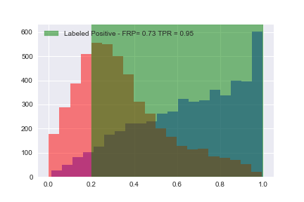
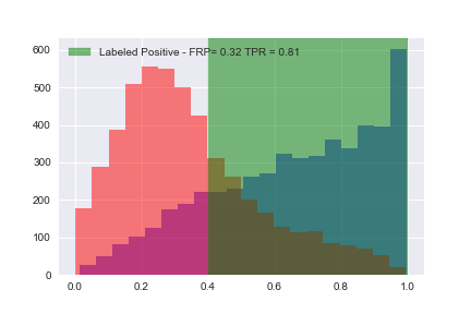
Let’s consider a concrete example where we use a very small fraction of the training data. The only purpose of this is to demonstrate the behavior of TPR and FPR as we modify the threshold for the model. We create some sample classification data:

from sklearn.datasets import make_classification
from sklearn.linear_model import LogisticRegression
import numpy as np
X, y = make_classification(n_samples=10000, n_features=10, n_classes=2, n_informative=5)
df_X=pd.DataFrame(X)
y_vals=np.array(y)
Xtrain = X[:9900]
Xtest = X[9900:]
ytrain = y[:9900]
ytest = y[9900:]

clf = LogisticRegression()
clf.fit(Xtrain, ytrain)

Now let’s add the actual outcome and score to a Pandas dataframe so we can study the results:

from sklearn import metrics
import pandas as pd
%matplotlib inline

df_X=pd.DataFrame(X)
df_X['score']=clf.predict_proba(df_X)[:,1]
df_X['outcome']=y_vals

Now that we have the dataframe, let’s plot the TPR and FPR as a function of our threshold:

import seaborn
import matplotlib.pyplot as plt
fprs=[]
tprs=[]
for i in range(0,11):
    threshold = float(i)/10
    print (threshold)
    fig, ax = plt.subplots()
    df_X[df_X['outcome']==1]['score'].hist(bins=20,color='b',alpha=0.5)
    df_X[df_X['outcome']==0]['score'].hist(bins=20,color='r',alpha=0.5)
    fpr = np.round(len(df_X[(df_X['outcome']==0) & (df_X['score']>threshold)])/len(df_X[df_X['outcome']==0]),2)
    tpr = np.round(len(df_X[(df_X['outcome']==1) & (df_X['score']>threshold)])/len(df_X[df_X['outcome']==1]),2)
    fprs.append(fpr)
    tprs.append(tpr)
    ax.axvspan(threshold, 1, alpha=0.5, color='g',label='Labeled Positive - FRP= ' + str(fpr)+' TPR = ' + str(tpr))
    plt.legend()
    plt.savefig("../img/roc_" + str(i) + ".png")
    plt.show()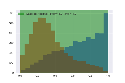

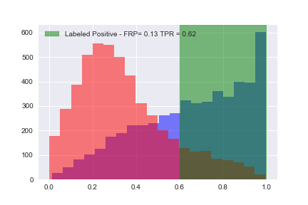
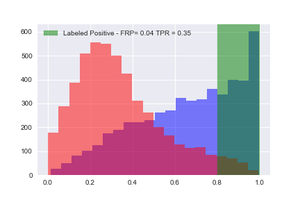
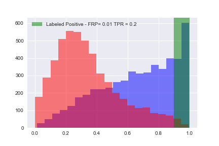
Now that we’ve calculated all of the tue positive rates (TPR) and false positive rates (FPR), let’s plot them:

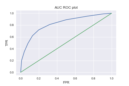
Conclusion: In general we always start off with a Bernoulli (or Multinomial in the case of multiple possible outcomes) prior and make certain simplifying assumptions about the underlying distribution. We observed that accuracy is not a good metric for evaluating classification models, and showed how AUC results in a bias-invariant estimate of the performance of your model.

Dorian Goldman

Introduction To Classification