So far all of the models we have considered have been parametric - ie. there is some underlying distribution with parameters \(\theta\) which we wish to learn. In this post, we will introduce Ensemble Methods which are non-parametric. In particular, we will cover Decision Trees and Random Forests. We will focus first on the case of classification.
Decision Trees
Constructing one tree
Let’s consider data \((\mathbf X, \mathbf y)\) where \(y \in \{0,1\}\). For classification, we seek a rule \(\mathbf x \mapsto p(\mathbf x)\) which maximizes:
\[\mathcal{L}(p) := \prod_{k=1}^N p(x_i)^{y_i} (1 - p(x_i))^{1-y_i}.\]Taking a log and dividing by \(N\) we have:
\[\mathcal{Q}(p) := \frac{1}{N}\sum_{k=1}^N y_i \log p(x_i) + (1-y_i)\log (1-p(x_i)).\]If we assume that \(x \mapsto p(x)\) is piecewise constant on regions \(S \subset X\) with value \(p(s)\), then notice that
\[\sum_{k=1}^N \frac{y_i}{N} \log p(s) = p(s) \log p(s).\]If we do this over the segments of \(X\) which componse the level sets of \(p\), then we have
\[\frac{1}{N}\sum_{k=1}^N y_i \log p(x_i) = \sum_{k=1}^N p(x_k) \log p(x_k).\]The calculation for the second term is similar, and optimizing \(p(X) \log P(X)\) is the same as \((1-P(X)) \log 1 - P(X)\). Thus if we constrain our functions to be piecewise constant, we wish to minimize the overall Entropy:
\[H(p) := \sum_{c=1}^M p_{c} \log p_c,\]where \(p_c = p(Y = c)\) and there are \(M\) possible classes. To get a sense of this term, observe that it is concave with maximum at \(\frac{1}{2}\) and \(H(0)=H(1) = 1\):
p = np.linspace(0.001,1,1000)
H = [-x*np.log(x) for x in p]
plt.plot(p,H)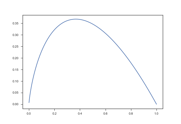
To fix ideas, we are going to use the Iris data set, which is a well known data set used to classify different types of flowers based on its size properties. It’s a good dataset to explain the fundamental principles of decision trees since there is a rich structure within a very small dataset.
Let’s load in the data and see what it looks like:
import seaborn as sns; sns.set(style="ticks", color_codes=True)
iris = sns.load_dataset("iris")
g = sns.pairplot(iris, hue="species")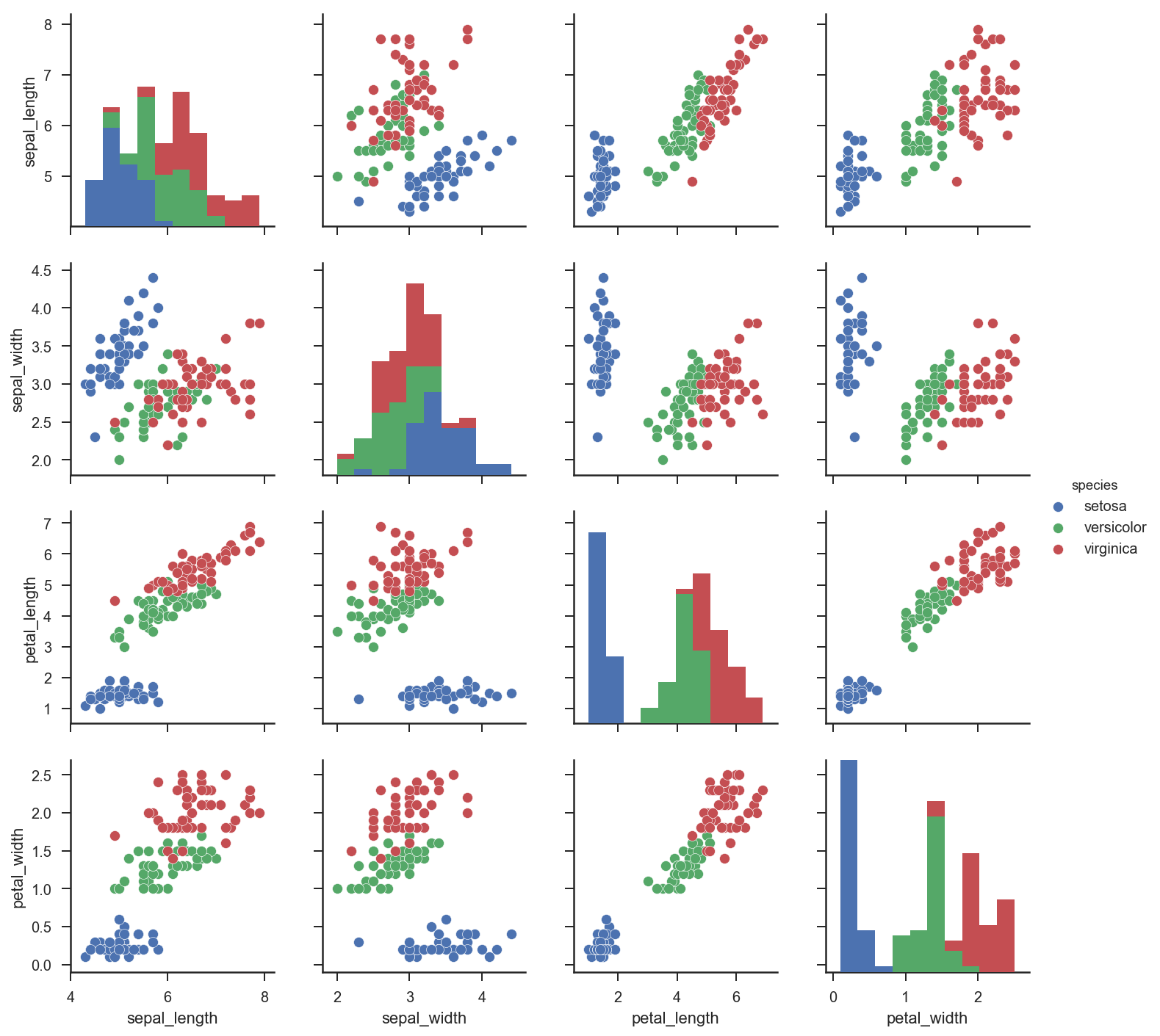
Decision Tree Algorithm
How do we minimize \(H\) above? In decision trees we use a forward greedy method. We will assume below our data is categorical. If it is not, then we assume we have applied some bucketing to the continous values.
First we compute the total entropy:
Step 1: Compute the total entropy of \(Y\).
\[H(P) = \sum_{c=1}^M p(Y=c) \log p(Y=c).\]This tells us how pure the classes are. In the Iris dataset above, we have \(M=3\) classes. Let’s compute this manually for Iris:
def entropy(y):
    classes = np.unique(y)
    size_classes = [len(y[y==c]) for c in classes]
    N = len(y)
    entropy = -np.sum([(s/N) * np.log(s/N) for s in size_classes])
    return entropy
entropy(iris['species'])Output:
1.0986122886681096Step 2: For each feature \(X_j\), compute conditional Entropy.
Let \(x_j^k\) be the values (or levels) that \(X_j\) takes on.
\[H(P | X_j) = \sum_{k=1}^{K_j} \sum_{c=1}^M p(Y=c | X_j=x_j^k) \log p(Y=c | X_j=x_j^k).\]We define the Information Gain of \(X_j\) as:
\[H(Y) - H(P | X_j).\]First we break our continous features into quantiles:
df_cat = pd.DataFrame(columns=iris.columns,index=range(len(iris)))
for feature in iris.columns.values[:-1]:
    df_cat[feature]=pd.qcut(iris[feature],4,range(4))

df_cat['species']=iris['species']
Next we will cycle through each feature and add up the entropies from each split to see which one is the best.
entropy_total = 0.0
entropies=[]
for feature in iris.columns.values[0:-1]:
    entropies=[]
    vals=np.unique(df_cat[feature].values)
    entropy_total = 0.0
    for t in np.unique(df_cat[feature].values):
        entropy_total = 0.0
        df_split1 = df_cat[df_cat[feature] <= t]
        df_split2 = df_cat[df_cat[feature] > t]

        if len(df_split1)>0:
            entropy_total = entropy_total + entropy(df_split1[feature])
        if len(df_split2)>0:
            entropy_total = entropy_total + entropy(df_split2[feature])
        entropies.append(entropy_total)

    plt.plot(vals,entropies,label=feature)
    plt.legend()
    plt.savefig(path + "entropy_iris_compare.png")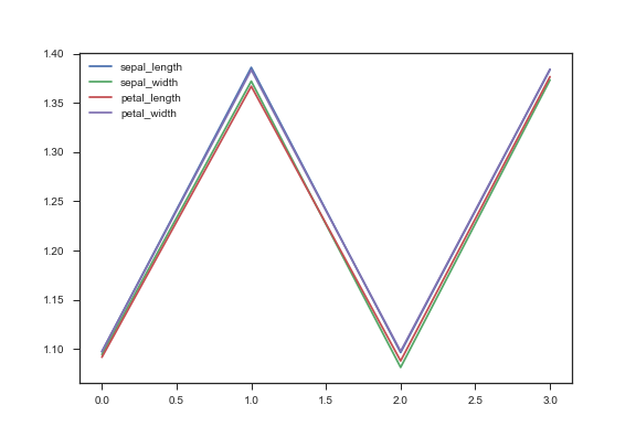
Printing the raw output we have:
Feature  sepal_length
[1.0972811987124906, 1.3859818285596666, 1.0964752493540126, 1.3839038058416437]
Feature  sepal_width
[1.0944710658789472, 1.3720185953928703, 1.0813741858392665, 1.3732786055462978]
Feature  petal_length
[1.0916813968397496, 1.366834096362366, 1.0879487948449884, 1.3765642287411282]
Feature  petal_width
[1.0975084815466807, 1.383434855088411, 1.0976531947932993, 1.3840689647011553]
Notice that it seems that the lowest entropy split (or highest information gain) is for the petal_length feature at the 25% threshold. Thus petal_length is our top feature.
Step 3: Pick \(X_*^1\) to be the feature which has largeest information gain and split.
We perform Step 2 for every \(X_j\), and choose our first feature be the solution of
\[X_*^1 := \textrm{argmax}_{j} H(Y) - H(P | X_j).\]Now split on \(X_*^1\) to be the optimal \(x_j^i\). In our case, the top feature was petal_length. Putting this into scikit-learn, we see it obtains the same result:
from sklearn.datasets import load_iris
from sklearn import tree
iris = load_iris()
clf = tree.DecisionTreeClassifier(max_depth=1)
clf = clf.fit(iris.data, iris.target)
dot_data = tree.export_graphviz(clf, out_file=None,
                         feature_names=iris.feature_names,
                         class_names=iris.target_names,
                         filled=True, rounded=True,
                         special_characters=True)
graph = graphviz.Source(dot_data)
graph 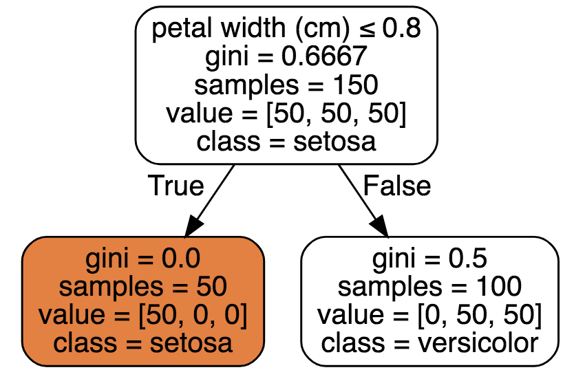
Step 4: Split on the above attribute and continue recursively.
Define
\(Y_1 := Y \lvert X_j = c_j^{*}\) and \(Y_2 = Y \lvert X_j \neq c_j^*\)
in the categorical case and
\(Y_1 := Y \lvert X_j >= c_j^{*}\) and \(Y_2 = Y \lvert X_j < c_j^*\)
in the continous case. Then repeat Step 2 with the new variables \(Y_1\) and \(Y_2\) recursively. Let’s just do one split to demonstrate how it works. Our best split was petal_width = 0 and petal_width > 0:
entropy(df_cat[df_cat['petal_length']==0]['species'])
Output:
0.0
Thus we have a pure branch on the second split!
Final decision tree code
Let’s now use sklearn to make the decision tree and plot it.
from sklearn.datasets import load_iris
from sklearn import tree
iris = load_iris()
clf = tree.DecisionTreeClassifier()
clf = clf.fit(iris.data, iris.target)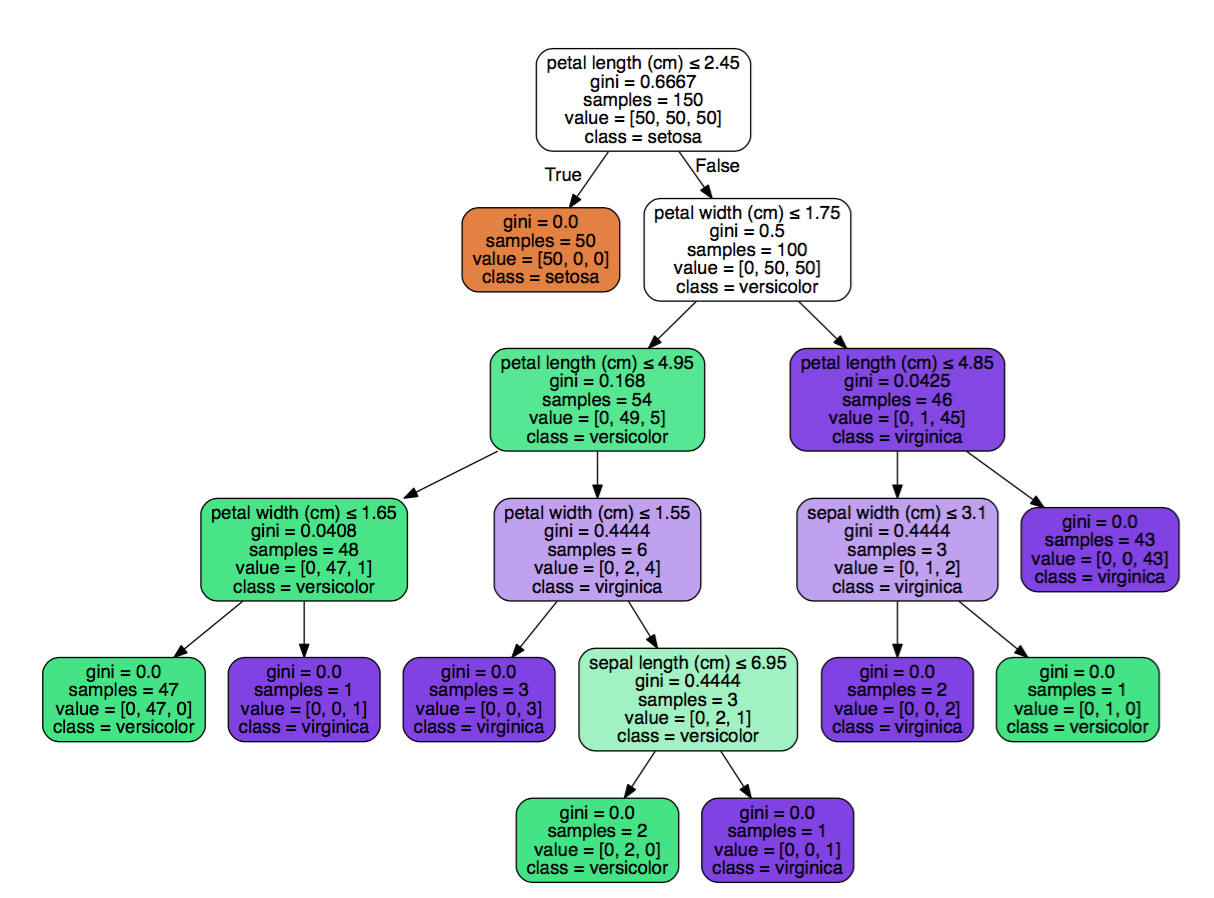
Notice how the decision tree found the same thing we did manually? petal_length is the top feature with a left split that has pure class.
Next: In our next post, we will cover ensemble methods, which combine many decision trees, or more generally, weak learners into one strong learner.