In this post, we will discuss Linear Regression. We will go over, in detail, the assumptions made for this model with some concrete examples. We will provide concrete examples of the failure of these assumptions and then discuss the lack of stability when you have correlated features.
In the next post, we will discuss model selection techniques and how to prevent over fitting by using various constraints on the coefficients.
Linear Regression
Most people are familiar with ordinary least squares. Given a collection of observations \(\{(y_i, \mathbf x_i)\}\), where \(\mathbf x_i \in \mathbb{R}^k\) are the features in our model, and \(\{y_i\}\) are the observed dependent variables, which we would like to model with \(\mathbf x_i\), we seek to find the \(\mathbf \beta \in \mathbb{R}^k\) which minimizes
\[\min_{\beta} \frac{1}{N} \sum_{i=1}^N(y_i - \beta \cdot \mathbf x_i)^2.\]Formally speaking, we are modeling our dependent variable \(Y\) as a linear function of the features \(X\) with some error. In other words,
\[Y - \beta \cdot \mathbf X \sim \epsilon(\beta)\]where \(\epsilon(\beta)\) is an error term which we would like to minimize. Less formally, the optimal \(\epsilon\) is a random variable which will have mean zero and some unknown variance.
In fact, for any kind of regression problem, we week to find \(f: \mathbf{X} \mapsto Y\) such that
\[Y - f(\mathbf{X}) \sim \epsilon(f).\]This seems pretty straightforward, right? The inquisitive may wonder the following:
- Don’t we want \(\epsilon (\beta)\) to be as close to zero as possible? What do we mean when we call this a random variable?
- Why do we use the \(L^2\) norm - is there a reason or advantage over using some other \(L^p\) space? In fact, why not replace \(L^2\) with any other appropriate metric \((y,\mathbf x) \mapsto d(x,\mathbf x)\)?
To answer the first question. Think of the following examples:
- Predicting the height of an individual based on age, gender and race. For a given combination (ie. (13, male, caucasian) ), we will have many possible values if we consider the entire population. There will be a fixed mean but it will vary.
- Predicting flight delays using the airline, destination, source location and weather. There will be many different time delays for any given combination of the above variables.
Thus we can’t actually expect to predict any exact value when considering stochastic values. The two main things we need to consider are:
- What distribution does \(p(y\rvert x,\beta)\) follow?
- What is the best choice of \(\beta\) given this prior?
Note: We have assumed here that the distribution is parametric, ie. \(\exists \beta\) such that the data is distributed via \(p(y\rvert x,\beta)\). For example
\[p(y \rvert x, \beta) = \frac{1}{\sqrt{2\pi \sigma^2}} e^{-\frac{(y-\beta \cdot x)^2}{2 \sigma^2}}.\]Why \(L^2\), why do we need all these assumptions below??
I find that many introductory articles/books on regression feel that students will be far too intimidated by probability to understand the idea of Maximum Likelihood. But without it, there is really no way to get a sense of what all the assumptions are that go into linear regressions, and why they are so important. For maximum likelihood, we wish to fit data to a prior distribution. More precisely, assuming an underlying distribution, can we solve:
\[\max_{\beta} \prod_{i=1}^Np(y_i | \beta_i,x_i) = \max_{\beta} \prod_{i=1}^N \frac{1}{\sqrt{2\pi \sigma^2}} e^{-\frac{(y_i-\beta \cdot x_i)^2}{2 \sigma^2}}.\]Noting that we can always compose any monotone function with an expression we are trying to maximize, we can take the log of the above function, which results (when the variances are equal!) in precisely
\[\min_{\beta} \frac{1}{N} \sum_{i=1}^N(y_i - \beta \cdot \mathbf x_i)^2.\]Note: This is where all of the assumptions come from below. I encourage the reader to think about how each one of the assummptions directly ties back to the assumption that \(y - \beta \cdot x\) is normally distributed with mean zero and constant variance.
Assumption 1 - Linear relationship between dependent and indepdent variables.
We assume that
\[Y = \beta \cdot \mathbf{X} + \epsilon ,\]where \(\epsilon\) is not influenced by \(\mathbf{X}\).
n = 5000
x = np.random.randn(n)
s = np.random.normal(0, 2, n)
yvals = [xval**2 + np.random.normal(0,1,1)[0] for xval in x]
y = 3*x +s

fig, ax = plt.subplots()
fit = np.polyfit(x, yvals, deg=1)
ax.plot(x, fit[0] * x + fit[1], color='red')
ax.scatter(x, yvals)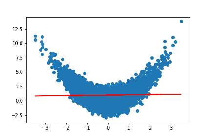
Assumption 2 - The residuals, \(\epsilon_i\), are i.i.d.
We assume that \(\epsilon_i := Y_i - f(\mathbf X_i)\) are all i.i.d random variables (indepdendent, identically distributed).
Note that it sufficies to assume independence of the error terms \(\epsilon_i\) to conclude that \(Y_i \rvert X_i\) are independent.
Indeed,
\[\mathbb{E}(Y \rvert X=x_i \cdot Y \rvert X = x_j) = \mathbb{E}( (\beta \cdot x_i + \epsilon_i) (\beta \cdot x_j + \epsilon_j)).\]Expanding, using the fact that \(x_i\) and \(x_j\) are deterministic so \(\mathbb{E}(x_i) = x_i\) and \(\mathbb{E}(x_j) = x_j\), along with independence of \(\epsilon_i\) and \(\epsilon_j\), so that
\(\mathbb{E}(\epsilon_i \epsilon_j) = \mathbb{E}(\epsilon_i) \mathbb{E}(\epsilon_j)\),
we have
\[\mathbb{E}(Y | X=x_i \cdot Y | X = x_j) = (\beta \cdot x_i + \mathbb{E}(\epsilon_i))(\beta \cdot x_j + \mathbb{E}(\epsilon_j)) = \mathbb{E}(Y \rvert X = x_i) \mathbb{E}(Y \rvert X=x_j).\]
n = 5000
x = np.random.randn(n)
s = np.random.normal(0, 2, n)
yvals = [3*xval + np.random.normal(0, xval**2,1)[0] for xval in x]
y = 3*x +s

fig, ax = plt.subplots()
fit = np.polyfit(x, yvals, deg=1)
ax.plot(x, fit[0] * x + fit[1], color='red')
ax.scatter(x, yvals)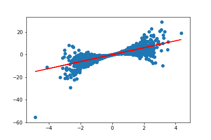
Assumption 2 - The residuals \(\epsilon_i\) are all normally distributed with zero mean, \(\epsilon_i \sim \mathcal{N}(0,\sigma^2).\)
Let’s take an example where we have a residual which has a non-zero mean, and see how scikit-learn learns the coefficients.
from sklearn import datasets, linear_model
regr = linear_model.LinearRegression()
n = 50000
x = np.linspace(0,1,n)
x_pd=pd.DataFrame(x,columns=['x'])
x_pd['const']=1
yvals = [xval + np.random.normal(10,2,1)[0] for xval in x]

# Train the model using the training sets
regr.fit(x_pd,yvals)

# Make predictions using the testing set
y_pred = regr.predict(x_pd)
plt.scatter(x,yvals)
plt.plot(x,x*regr.coef_[0] + regr.coef_[1],color='r')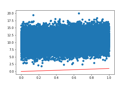
What went wrong here? Let’s check the coefficients:
regr.coef_We obtain the following model:
\[\hat y = 1.03 x.\]The model got the linear coeffficient correct, but scikit-learn assumes that the data has been mean centered before training by default. If we want to correct this issue, we can add fit_intercept=False:
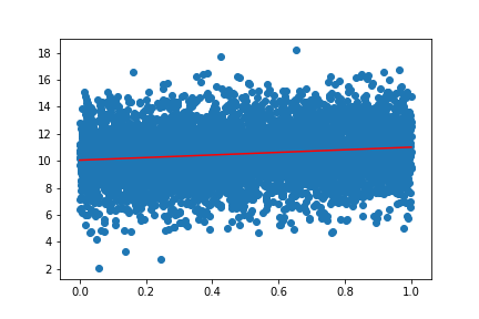
regr = linear_model.LinearRegression(fit_intercept=False)
Then we obtain:
Assumption 3 (not technically necessary) - The matrix \(\mathbf{X^TX}\) has full rank.
Using Calculus, we obtain the general solution when \(X^TX\) is invertible:
\[\hat \beta = (X^TX)^{-1} X^T y.\]When it’s not, we can still minimize the \(L^2\) norm of the residuals, but we lack stability. To see why, a simple computation shows that:
\[\frac{d^2}{d\beta^2} \sum_i (y_i - \mathbf{\beta} \cdot \mathbf{x_i})^2 = \frac{2}{N} X^TX.\]From what we know about linear algebra, this matrix is positive semi-definite and symmetric. It is positive definite precisely when the columns of \(X\) are linearly independent (ie. the features aren’t correlated). Let’s simulate two correlated features with noise \(x_1\) and \(x_2\) with a well defined linear trend:
\[y = x_1 + \epsilon,\]where \(\epsilon \sim \mathcal{N}(0,0.01)\) and see how stable the coefficients are:
Correlated Features
n=10000
x1 = np.linspace(0,0.01,n)


s = np.random.normal(0, 0.001, n)

x2 = 100*x1 + s

df=pd.DataFrame({'x1':x1,'x2':x2})

y = x1 + np.random.normal(0, 0.01, n)
coefs1=[]
coefs2=[]
scores_perp=[]
for i in range(0,100):
    y = x1 + np.random.normal(0, 0.001, n)
    regr = linear_model.LinearRegression()
    x=df
    # Train the model
    regr.fit(x,y)
    coefs1.append(regr.coef_[0])
    coefs2.append(regr.coef_[1]*100)
    scores_perp.append(regr.score(x,y))

plt.figure(figsize=(8,5))
plt.plot(coefs1,label='x1')
plt.plot(coefs2,label='x2')
plt.legend()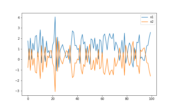
Orthogonal Features
Now let’s check the same model with \(x_1 \perp x_2\).
from numpy import linalg as LA
n=10000
x1 = np.linspace(0,0.01,n)


k = np.random.normal(0,0.01,n)/np.linalg.norm(k)**2
s = np.random.normal(0, 0.001, n)

x2 = 100*np.linspace(0,0.01,n)
x2 -= x1.dot(k) * k / np.linalg.norm(k)**2
x1=k
df=pd.DataFrame({'x1':x1,'x2':x2})

y = x1 + np.random.normal(0, 0.01, n)
coefs1=[]
coefs2=[]
scores_perp=[]
for i in range(0,100):
    y = x1 + np.random.normal(0, 0.001, n)
    regr = linear_model.LinearRegression()
    x=df
    # Train the model
    regr.fit(x,y)
    coefs1.append(regr.coef_[0])
    coefs2.append(regr.coef_[1]*100)
    scores_perp.append(regr.score(x,y))

plt.figure(figsize=(8,5))
plt.plot(coefs1,label='x1')
plt.plot(coefs2,label='x2')
plt.legend()
plt.show()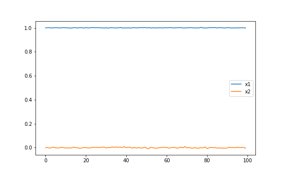
We see from the above two scenarios that the coefficients are much more stable when we have orthongla features. Let’s actually plot Hessian of the objective function for \(\mathbf{X} = [\mathbf{x_1} \mathbf{x_2}]\) in the two cases.
Correlated Features
xlist = np.linspace(0, 1.0, 100) # Create 1-D arrays for x,y dimensions
ylist = np.linspace(0, 1.0, 100)

A=df.corr()
X,Y = np.meshgrid(xlist,ylist)
plt.figure(figsize=(8,8))
A=df.corr()
Z = A.loc['x1','x1']*X**2 + 2*X*Y*A.loc['x1','x2'] + A.loc['x2','x2']*Y**2
plt.contour(X, Y, Z, [0.5, 1.0, 1.2, 1.5], colors = 'k', linestyles = 'solid')
plt.savefig("/Users/dgoldma1/Documents/doriang102.github.io/img/perpellipse.png")

plt.show()
Running the same code on the Hessian of the orthogonal features, we obtain:
Orthogonal Features
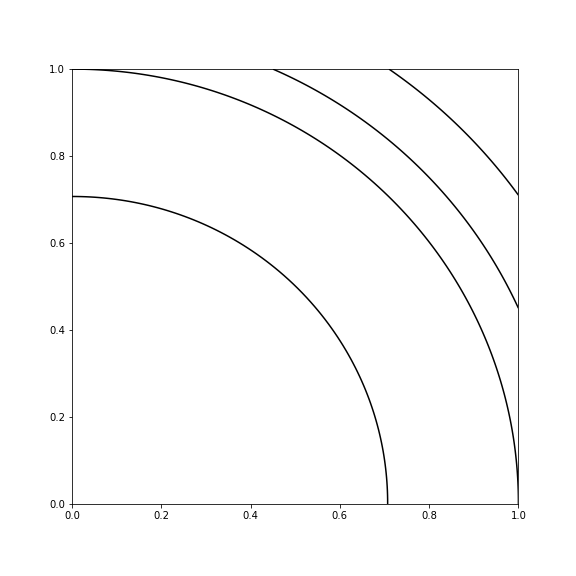
Notice how in the correlated case, there is clear degeneracy - the solution is not unique. Any value along that line is constant, so there is no unique solution. This is what accounts for the instability in the solution.
Fixing the issue using regularization.
We will cover this in the next section, but one simple way to make the OLS problem well posed is to add in a convex penalization term:
\[\min_{\beta} \frac{1}{N} \sum_{i=1}^N(y_i - \beta \cdot \mathbf x_i)^2 + \lambda \|\beta\|_{L^p}.\]For \(p > 1\), this problem is now strictly convex even with correlated features, and thus there is a unique solution, which for \(p=2\) is:
\[\beta^* = (X^TX + \lambda I)^{-1} X^T y.\]Conclusion
In this post we’ve seen that essential ingredients for the linear regression problem to be well posed are:
- 1) The outcome variable \(y\) follows a linear trend with the data \(X\).
- 2) The residuals, \(y - \beta \cdot \mathbf{x}\) are normally distributed with mean zero and constant variance.
- 3) Correlated features don’t preclude the existence of solutions to the linear regression problem, but they cause issues with instability of the coefficients, and can potentially impact perfomance. We can fix this via regularization though, and we will cover this in the next post.
In the next post, we will look into methods of regularization and how it can help with over fitting models. We will also look at standard data preparation techniques that are needed for regularization, or any kind of interpretability even without regularization.
Common Confusions:
- 1) Some beginningers think that the features themselves need to be normally distributed, or that \(y\) does, this is false.
- 2) Your data does not need to be normalized for the problem to be well posed, but as we will see in the next section, interpretiability is impacted if you don’t, and it’s very important if you are performing regularization methods (which is almost always the case).