In this section, we look more carefully at the sample size necessary to make statistically valid inferences from observations, and see what estimates we obtain on our confidence of the outcome for both Frequentist and Bayesian approaches.
When organizing an experiment, we must ask ourselves a few questions (not exhaustive):
-
1) What is the hypothesis we are testing?
-
2) How big of a sample size do we need to read results in a statistically meaningful way?
-
3) What would be considered a ‘positive’ result?
In this post, we will focus on 2) and 3). First, we outline the frequentist approach, then the Bayesian approach. We will see that the sample size needed to make inferences scales in identical ways even though they are two entirely different ways of thinking about the problem of inference. I personally feel that the Bayesian approach is more natural, and make a case for this in the second section.
We reconsider the example of the two buttons outlined in the first blog post Hypothesis Testing. If you haven’t read this already, I highly recommend you skim it in order to be familiar with the notation/ideas in this post.
Frequentist Statistical Power
In the frequentist approach, as we saw in the last section, we wish to estimate the probability of making an observation at least as large as the difference observed under the assumption that the two buttons are identical.
For statistical power in the frequentist setting, we ask:
Question: What is the required sample size to reject the null hypothesis assuming that the two buttons are different?
Mathematically this is expressed as:
\[p(\textrm{reject } H_0 \rvert H_1 \textrm{ is true}).\]In other words, what’s the probability we will be able to reject the null hyothesis if the difference we observe is actually true? If we reject the null hypothesis at a p value of \(0.05\) for instance, and we know that button 1 out performs button 2 by some threshold \(\alpha\), how many observations would we need to be 95% sure that this result is true?
Let’s define some quantities:
-
Let’s set \(p_1 - p_2 = \alpha > 0\).
-
\(N_1 = N_2=N\) are the sample sizes of the experiment (set equal for simplicity).
-
\(z_{\alpha}\) is the minimum z score we need to have the probability of observing \(\alpha\) to be under the necessary threshold. For \(0.05\), \(z_{\alpha}=1.645\) for example.
Then we have
\[p(\textrm{reject } H_0 \rvert H_1 \textrm{ is true}) = p(z > z_{\alpha} \rvert p_1-p_2 = \alpha).\]From the last section, we can write this as
\[\frac{ p_1 - p_2 }{\sqrt{ p_1(1-p_1)/N + p_2(1-p_2)/N}} > z_{\alpha}.\]Since \(p_1 - p_2 = \alpha\) and \(\alpha\) is generally much smaller than both \(p_1\) or \(p_2\), we can set \(p_1 \sim p_2 := p\) in the denominator to obtain
\[\frac{N\alpha^2}{2p(1-p)} > z_{\alpha}^2.\]Rewriting this we obtain
\[N \geq 2 \frac{\sigma^2 z_{\alpha}^2 }{\alpha^2},\]where \(\sigma^2\) is the variance of the expected baseline conversion rate. In particular, when \(z_{\alpha}=1.65\), we have
\[N \geq 5.44 \frac{\sigma^2 }{\alpha^2}\]To see what different sample sizes we need, let’s plot some of these curves.
First, let’s write a formula to compute the p value of the difference between two conversion rates. We first define:
import scipy.stats as st
def p_value(p_T,p_C,size_T,size_C):
    var = np.sqrt(p_T*(1-p_T)/size_T + p_C*(1-p_C)/size_C)
    diff = p_T-p_C
    z_score = diff/var
    p_value = st.norm.sf(abs(z_score))
    return diff, p_value
p_values=[]
diffs=[]
Let’s then compare a list of p values of different scales:
N_vals_1 = [5.44*(p*(1-p))/((0.01*p)**2) for p in p_conv]
N_vals_5 = [5.44*(p*(1-p))/((0.05*p)**2) for p in p_conv]
N_vals_10 = [5.44*(p*(1-p))/((0.10*p)**2) for p in p_conv]
N_vals_20 = [5.44*(p*(1-p))/((0.20*p)**2) for p in p_conv]

plt.figure(figsize=(8,8))
plt.xlabel('Conversion Rate')
plt.ylabel('Required Sample Size for p < 0.05')
plt.plot(p_conv,N_vals_5,label='5% lift')
plt.plot(p_conv,N_vals_10,label='10% lift')
plt.plot(p_conv,N_vals_20,label='20% lift')
plt.legend()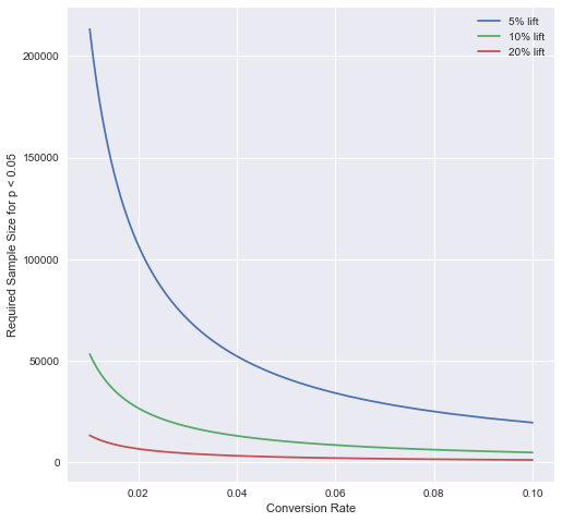
In my experience, one is generally looking for lifts of the order of \(1-2\%\), so you can see how the sample size is incredibly important. Generally major websites can have of the order of 20 to 100 million unique cookies visit every month, and can have anywhere from 50k to 1 million actual users.
Bayesian Statistical Power
For statistical power in the Bayesian setting, we ask:
Question: What is the required sample size to be 95% sure that \(p_1 > p_2\)?
I personally find this question much more ‘natural’. We focus here on the case of a uniform prior on the outcomes, and will possibly study later the effects of different priors on the sample size. Although it is clear from this discussion that the more we know in the beginning, smaller \(N\) we need to draw conclusions. There is always a risk that our prior is wrong though, so we are safe in choosing a uniform one.
We’ll see in this post that the distributions of outcomes concentrate as (asymptotically) Gaussians around the observed success frequency. We will work to estimate:
\[P[p_1 > p_2 | D_1,D_2] \sim \int_{p_1>p_2} \delta_{\beta_1}(p_1) \delta_{\beta_2}(p_2),\]where \(\delta_{\beta_i}\) like a mollified dirac measure concentrated at \(\beta_i\) in the form of a narrow Gaussian.
We will estimate \(p_1 > p_2\) when \(\beta_1 < \beta_2\) from above and see that it is an integral over the red shaded region of the blue triangle in the plot below, which is expnentially small in \(\sqrt{N}\) as \(N \to +\infty\):
import matplotlib.pyplot as plt
import numpy as np

X = np.linspace(0, 1, 100)
Y = np.linspace(0, 1, 100)

x,y = np.meshgrid(X,Y)

f1 = (1/(2*np.pi*sigma_x*sigma_y) * np.exp(-((x-0.8)**2/(2*sigma_x**2)
     + y**2/(2*sigma_y**2))))
f2 = (1/(2*np.pi*sigma_x*sigma_y) * np.exp(-((x-0.4)**2/(2*sigma_x**2)
     + y**2/(2*sigma_y**2))))

plt.contour(x,y,f2,cmap='Reds')
plt.contour(x,y,f1,cmap='Blues')
plt.contour(y,x,f2,cmap='Reds')
plt.contour(y,x,f1,cmap='Blues')
plt.fill_between(x[0],x[0],1,where=x[0] >= 0.6, facecolor='blue', interpolate=True,alpha=0.1)
plt.plot(X,X)
plt.show()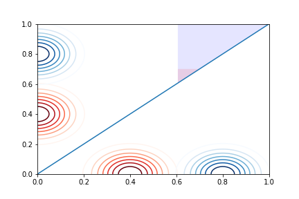
We will see that
\[N \geq \frac{C(\sigma_{\beta_1}^2 + \sigma_{\beta_2}^2)}{\alpha^2} \log \frac{1}{p_{\min}},\]where \(p_{\min}\) is the minimum probability (ie. \(0.95\)) we require to be confident of our result.
Main results
We saw in the last post that
\(p^n (1-p)^{N-n} \to \delta_{\frac{n}{N}}(p),\) in the sense of distributions. How do we infer confidence in the Bayesian setting? Let’s now assume that we have \(\beta = \frac{n}{N}\) successes.
With what confidence can we infer that the button has bias $\beta$?
Let’s define
\(H_1\) - The hypothesis that \(p_1 = p_2\).
\(H_2\) - The hypothesis that \(p_1 > p_2\).
We can first consider the Baye’s ratio:
\(\frac{p(D \lvert H_1)}{p(D \lvert H_2)}.\) We can write this as
\[\frac{p(D \lvert H_1)}{p(D \lvert H_2)} = \frac{(\beta+\epsilon)^n (1- (\beta+\epsilon))^{N-n} }{ \beta^n (1- \beta)^{N-n}}.\]Lemma 1: Let \(\beta = \frac{n}{N}\). Then it holds that
\[\frac{p(D \lvert H_1)}{p(D \lvert H_2)} = e^{\frac{-N c_{\beta,\epsilon} \epsilon^2}{\sigma_{\beta^2}}},\]where \(\sigma_{\beta} = \beta (1- \beta)\) _and \(c_{\beta,\epsilon}\) is a constant satisfying
\[\frac{1}{4} \leq c_{\beta, \epsilon} \leq 1.\]Proof:
Let’s take the log of the ratio above. Then we have
\[\frac{1}{N} \log \left(\frac{p(D \lvert H_1)}{p(D \lvert H_2)}\right) = \beta \log \left(1+ \frac{\epsilon}{\beta}\right) + (1-\beta) \log \left ( 1 - \frac{\epsilon}{1-\beta}\right).\]We expand the logs to second order via Taylor series with remainder to obtain:
\[\frac{1}{N}\log \left(\frac{p(D \lvert H_1)}{p(D \lvert H_2)}\right) = -\frac{c_{\epsilon,\beta} \epsilon^2}{2\beta} - \frac{\tilde c_{\epsilon,\beta}\epsilon^2}{2(1-\beta)} .\]Since we have
\[\frac{d^2}{dx^2} \log (1 + x) = - \frac{1}{1+x^2},\]by Taylor’s formula we can bound \(c_{\epsilon,\beta}\) and \(\tilde c_{\epsilon,\beta}\) by:
\[\frac{1}{4} \leq c_{\alpha, \beta}, \tilde c_{\alpha, \beta} \leq 1.\]Thus we have
\[-\frac{c_{\epsilon,\beta} \epsilon^2}{2\beta} - \frac{\tilde c_{\epsilon,\beta}\epsilon^2}{2(1-\beta)} = -\left(\beta c_{\epsilon,\beta} + (1-\beta) \tilde c_{\epsilon,\beta}\right) \frac{\epsilon^2}{2\sigma_{\beta}^2}.\]Simplifying, and changing the constant \(c_{\beta, \epsilon}\), the right side becomes
\[-\frac{c_{\beta,\epsilon} \epsilon^2}{2\sigma_{\beta}^2}.\]Taking the exponential completes the argument.
Q.E.D.
Thus we have immediately from the above the following Corollary.
Corollary 1: Let
\[R := \frac{p(D \lvert H_1)}{p(D \lvert H_2)} \leq e^{-\frac{N \epsilon^2}{8\sigma_{\beta}^2}}.\]Then we have
\[N \geq \frac{8\sigma_{\beta}^2}{\epsilon^2} \log \frac{1}{R}.\]What we really want to estimate is
\[\frac{\int\int_{p_1 > p_2} p_1^{n_1} (1-p_1)^{N-{n_1}} p_2^{n_2} (1-p_2)^{N-n_2} dp_1dp_2}{\int \int p_1^{n_1} (1-p_1)^{N-n_1} p_2^{n_2} (1-p_2)^{N-n_2} dp_1dp_2}\]We can rewrite the numerator as
\[\int_0^1 p_2^{n_2} (1-p_2)^{N-n_2} \int_0^{p_2} s^{n_1} (1-s)^{N-n_1} ds dp_2.\]Separating the denominator out, we have
\[\frac{1}{B(n_2+1,N-n_2-1)}\int_0^1 \Phi_{n_1}(p_1) p_2^{n_2} (1-p_2)^{N-n_2} dp_2.\]Let’s start off with an easier Lemma though.
Theorem 2: Let
\[\Phi_n(x) := \frac{\int_0^x p^n (1-p)^{N-n}}{\int_0^1 p^n (1-p)^{N-n}}.\]Then we have for \(\lvert x - \beta \rvert > \alpha\),
\[\lvert \Phi_n(x) - \mathbf{1}[\beta,1) \rvert \leq 2e^{-\frac{N\alpha^2}{\sigma_{\beta}^2}},\]and \(\Phi_n(\beta) \to 1/2\) exponentially fast.
Proof:
Courtesy of Lemma 1, we can write the function as
\[\Phi_n(x) := \frac{\int_0^x e^{-N\frac{c_{\epsilon,\beta} (p-\beta)^2}{\sigma_{\beta}^2}}dp}{\int_0^1 e^{-N\frac{c_{\epsilon,\beta} (p-\beta)^2}{\sigma_{\beta}^2}}dp}.\]Let’s introduce the change of variables
\[y = \frac{\sqrt{N c_{\epsilon,\beta}} (p-\beta)}{\sigma_{\beta}}.\]Then we have
\[\Phi_n(x) = \frac{\int_{-\frac{\sqrt{Nc_{\epsilon,\beta}}\beta}{\sigma_{\beta}}}^{\frac{\sqrt{Nc_{\epsilon}}(x-\beta)}{\sigma_{\beta}}} e^{-y^2} dy}{\int_{-\frac{\sqrt{Nc_{\epsilon,\beta}}\beta}{\sigma_{\beta}}}^{\frac{\sqrt{Nc_{\epsilon}}(1-\beta)}{\sigma_{\beta}}} e^{-y^2} dy}\]Using the stanard Calculus trick of changing to polar coordinates, we can bound the Guassian integral:
\[\sqrt{2\pi} \sqrt{ 1 - e^{-a^2}} \leq \int_{-a}^a e^{-y^2} dy \leq \sqrt{2\pi} \sqrt{1 - e^{2a^2}},\] \[\int_{a}^{+\infty} e^{-y^2} dy \leq \sqrt{2\pi} e^{-a^2}.\]Using this we obtain the bound for \(x < \beta - \alpha\):
\[\Phi_n(x) \leq \frac{ e^{-N c_{\epsilon}^2 \alpha^2/\sigma_{\beta}^2}}{\sqrt{1 - e^{-N c_{\epsilon,\beta}^2\beta^2/\sigma_{\beta}^2}}} \leq 2e^{-N c_{\epsilon}^2 \alpha^2/\sigma_{\beta}^2}\]For \(x > \alpha + \beta\),
\[\Phi_n(x) \geq \frac{ \sqrt{1 - e^{-N c_{\epsilon,\beta}^2 \alpha^2/\sigma_{\beta}^2}}}{\sqrt{1 - e^{-N c_{\epsilon,\beta}^2\beta^2/\sigma_{\beta}^2}}} \geq 1 - e^{-N c_{\epsilon,\beta}^2\beta^2/\sigma_{\beta}^2}.\]Q.E.D
From this we can estimate:
\[\frac{1}{B(n_2+1,N-n_2-1)}\int_0^1 \Phi_{n_1}(p_2) p_2^{n_2} (1-p_2)^{N-n_2} dp_2.\]By using Theorem 2, if we assume \(\beta_1 - \beta_2 > \alpha\), we have for a universal constant \(C>0\)
\[P(p_1 > p_2) \geq \mathbf{1}[\beta_2, 1)(\beta_1) - C e^{-N\alpha^2}{\sigma_{\beta}^2} = 1-C e^{\frac{-N\alpha^2}{\sigma_{\beta}^2}} .\]Thus if we wish to be 95% sure that \(p_1 > p_2\), as before we can compute:
\(1-C e^{\frac{-N\alpha^2}{\sigma_{\beta}^2}} \geq 0.95\).
Rearranging this, we obtain:
\[N \geq \frac{C\sigma_{\beta}^2}{\alpha^2} \log \frac{1}{0.95}.\]