In this first blog post, I plan on discussing the detailed mathematics behind A/B testing using both a frequentist and bayesian approach. Here is a broad summary before we get into more detail:
Let’s assume that we have two buttons, a red button and a blue button. We wish to construct a proper experiment to test out which button results in higher conversions (clicks/likes, etc).

Let \(X_i^R\) and \(X_i^B\) be the outcomes of the \(ith\) observation for the red and blue buttons respectively, ie. \(X_i^{R,B} = 1\) if the user clicked the button, and \(X_i^{R,B} = 0\) otherwise. Then we define the number of clicks of the red and blue buttons after \(N_R\) and \(N_B\) respective trials:
\[S_N^R = \sum_{i=1}^{N_R} X_i^R\] \[S_N^B = \sum_{i=1}^{N_B} X_i^B.\]Frequentist approach: Make no prior assumptions about what the parameters are, but use the asymptotic convergence of a sequence of independent Bernoulli trials to the normal distribution to compute the probability of observing a difference equal to or larger than that observed, under the null hypothesis, ie. assuming the two samples come from the same underlying distribution. What I will show however, is that frequentists ultimately have to assume a prior assumption on the data in order to computea p value with any kind of asymptotic certainty. I’m not sure I’ve seen this emphasized in the literature, so I want to bring it to people’s attention here.
Bayesian approach: Given a prior distribution on the possible means, update the posteriors based on Bayes formula, and compute the proabbility that \(p_1 > p_2\) over the range of all possible values of \(p_R\) and \(p_B\) (ie. don’t just assume there is one fixed value). The only criticism I’ve seen of this method is the assumption of a prior, however, as we will see, the frequentists also make this assumption if they want to have a correctly evaluated p value.
Frequentist Appraoch - p values and asymptotic normality
Let’s begin by the assumptions that the frequentist makes:
We make the following assumptions:
- Both \(\{X_i^R\}\) and \(\{X_i^B\}\) form a collection of independent, identitically dstirbuted random variables (i.i.d).
- Moreover, for each \(i\), \(X_i^R\) and \(X_i^B\) are sampled from fixed Bernoulli distributions with means \(p_R\) and \(p_B\) respectively.
As a result of the Law of Large Numbers, we have \(\frac{1}{N_R}S_N^R \to p_R\) and \(\frac{1}{N_B}S_N^B \to p_B\) as \(N_R,N_B \to +\infty\) in probability.
The Central Limit Theorem tells us the next order correction term is actually normal:
\[\frac{1}{\sqrt{N_R}} \sum_{i=1}^{N_R} X_i^R \to \mathcal{N}(p_R, \sqrt{p_R(1-p_R)})\] \[\frac{1}{\sqrt{N_B}} \sum_{i=1}^{N_B} X_i^B \to \mathcal{N}(p_B, \sqrt{p_B(1-p_B)})\]Another way to write the above is
\[\frac{1}{N_R}\sum_{i=1}^{N_R} X_i^R - p_R + E_1 \sim \mathcal{N}\left(0, \frac{p_R(1-p_R)}{N_R}\right)\] \[\frac{1}{N_B}\sum_{i=1}^{N_B} X_i^B - p_B + E_2 \sim \mathcal{N}\left(0, \frac{p_B(1-p_B)}{N_B}\right),\]where \(E_1\) and \(E_2\) are errors that tend to \(0\) as \(N_R, N_B \to +\infty\).
We’ve make use of the following facts:
- We can absorb the \(\sqrt{N_R}\) and \(\sqrt{N_B}\) terms into the variances of the normal distributions.
- The difference of two normally distributed random variables \(\mathcal{N}_1(\mu_1,\sigma_1)\) and \(\mathcal{N}_2(\mu_2,\sigma_2)\) is again a normally distributed random variable with mean \(\mu_1 - \mu_2\) and variances \(\sigma_1^2 + \sigma_2^2\).
Let’s plot the Binomial distributions and see how the red and blue button distributions look for fixed values:
import numpy as np; np.random.seed(10)
import seaborn as sns; sns.set(color_codes=True)

# Set number of observations.
n_R=1000
n_B=1200

# Set conversion rates of observations.
p_R=0.1
p_B=0.12

# Set number of samples to take
samples=10000

# Sample from red and blue butotn given observed conversion rates.
x_R = np.random.binomial(n_R, p_R, samples)/n_R
x_B = np.random.binomial(n_B, p_B, samples)/n_B

# Create pandas series
x_R=pd.Series(x_R)
x_B=pd.Series(x_B)

# Plot the results.
x_B.plot(kind='kde',label='Blue Button',color='b')
x_R.plot(kind='kde',label='Red Button',color='r')
sns.distplot(x_R,kde=False,norm_hist=True)
sns.distplot(x_B,kde=False,color='r',norm_hist=True)


x_position = 0.11
plt.axvline(x_position)
plt.legend()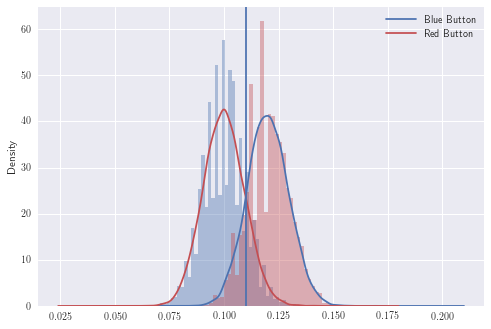
These distributions look approximately normal which is good. Now to continue with the frequentist approach, we need to introduce the null hypothesis.
Null Hypothesis: We assume that \(p_B = p_R\). How probable is our observed result?
Under this assumption, we can take the difference of the two sums, and normalize to obtain:
\[\frac{\frac{1}{N_R}\sum_{i=1}^{N_R} X_i^R - \frac{1}{N_B}\sum_{i=1}^{N_B} X_i^B}{(1/\sqrt{N_R})\sqrt{ p_R(1- p_R)} +(1/\sqrt{N_B})\sqrt{ p_B(1- p_B)}} + E_4 \sim \mathcal{N}(0,1),\]where \(E_4 \to 0\) as \(N_R,N_B \to +\infty\).
Now we do not know \(p_R\) or \(p_B\), even when we assume they’re equal.
However we have the following:
\[\frac{1}{N_R} \sum_{i=1}^{N_R} X_i^R = \hat p_R\] \[\frac{1}{N_B} \sum_{i=1}^{N_B} X_i^B = \hat p_B,\]which, courtesy of the fact that that \(\hat p_R \to p_R\) and \(\hat p_B \to p_B\) in probability, we can replace \(p_R\) and \(p_B\) with \(\hat p_R\) and \(\hat p_B\) by absorbing the error into \(E_4\).
Let’s now simulate this with fixed \(p_B\) and \(p_R\)
# Set number of observations.
n_R=100
n_B=120

for f in range(1,5):
    n_R = n_R*f
    n_B = n_B*f
    # Set conversion rates of observations.
    p_R=0.1
    p_B=0.12

    # Set number of samples to take
    samples=10000

    x_null=np.random.normal(0, np.sqrt(p_R*(1-p_R)/n_R) + np.sqrt(p_B*(1-p_B)/n_B), samples)

    # Create pandas series
    x_null=pd.Series(x_null)
    plt.xlim([-0.5,0.5])

    # Plot the distribution
    x_null.plot(kind='kde',label='N=' + str(n_R),color='g')
    sns.distplot(x_null,kde=False,norm_hist=True)

    # Plot the observed difference of p_B-p_R.
    x_position = 0.02
    plt.axvline(x_position)

    plt.legend()
    plt.show()
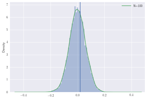
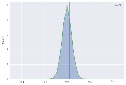
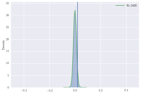
The area to the right of the line is the probability of observing the difference we have or larger, under the null hypothesis. In other words, it is the probability of observing any \(z \geq z_n\) from \(\mathcal{N}(0,1)\) where
\[\hat z_N = \frac{\hat p_R - \hat p_B}{(1/\sqrt{N_R})\sqrt{ \hat p_R(1- \hat p_R)} +(1/\sqrt{N_B})\sqrt{ \hat p_B(1- \hat p_B)}}.\]This is preceily the p value, ie.
\[p = \Phi( z \geq z_n),\]where \(\Phi\) is a standard unit normal.
However notice that we’ve just conveniently skipped over the error \(\tilde E_4\), which there are no currently known estimates for that don’t depend on initial ‘priors’ on \(p_R\) and \(p_B\). For this reason, I would take p values for Bernoulli trials with a grain of salt.
What we really need is the Berry-Esseen theorem which, under certain assumptions, gives a rate of convergence to a normal distribution. In particular, if we have
\[\mathbb{E}(|X_1|^3) := \rho < +\infty\]then it follows that
\[\left|F_{n}(x)-\Phi (x)\right| \leq \frac{C\rho}{\sigma^3 \sqrt{n}},\]where \(F_n(x)\) is the cumulative distribution function of \(\frac{1}{\sqrt{n}\sigma} \sum_{i=1}^N X_i\).
Nobody yet has been able to prove what the optimal constant is! The best estimate as of 2012, is C < 0.4748 and is due to due to Shevtsova (2011)
Special case of Bernoulli random variable
Note that for a Bernoulli random variable with parameter \(p\), it is clear that
\[\mathbb{E}(|X_1|^3) = p.\] \[\sigma^3 = p^3(1-p)^3\]which results in a best upper bound of
\[\left|F_{n}(x)-\Phi (x)\right| \leq \frac{0.48}{p^2(1-p)^3 \sqrt{n}},\]Thus we can only compute p values if we bound the range of possible means to begin with! This is essentially the same as assuming a Bayesian prior in the first place!
This is why I beleive much more in Bayesian methods. They are simpler, more natural, and don’t rely on any mysterious asymptotic approxmiations.
Bayesian Approach - Distribution on Parameters
The Bayesian approach says we don’t know what the means are for the red and blue buttons, but let’s assume they have some prior distribution (say uniform, if we have no idea), ie. \(F(p_R) = F(p_B) = 1\), and let’s try to infer the parameters by Bayes rule using the data observed.
Once again, let \(X_i^R\) and \(X_i^B\) be the outcomes of the \(ith\) observation for the red and blue buttons respectively, ie. \(X_i^{R,B} = 1\) if the user clicked the button, and \(X_i^{R,B} = 0\) otherwise.
Our goal is to determine:
\[p(p_B > p_R | D_R, D_B)\]where \(D_R\) and \(D_B\) represent the observations for the red and blue buttons respectively. One can compare this to the frequentist approach which essentially tries to infer:
\[p(D_R, D_B|p_B = p_R)\]How do we infer \(p(p_B > p_R \rvert D_R, D_B)\)? Let’s use Bayes theorem:
\[p(p_B > p_R | D_R, D_B) = \frac{\int_0^1 \int_0^1 I(p_B > p_R) P[D_B|p_B] P[D_R|p_R] dF_R(p_R) dF_B(p_B)}{\int_0 ^1 \int_0^1 P[D_B|p_B] P[D_R|p_R] dF_B(p_B) dF_R(p_R) }\]How do we determine \(p[D_B \rvert p_B]\) and \(p[D_R \rvert p_R]\)? Since this is a Bernoulli distribution, we have
\[p[D_B \rvert p_B] = {n_B \choose k_B} p^{k_B} (1-p)^{n_B-k_B}\] \[p[D_R \rvert p_R] = {n_R \choose k_R} p^{k_R} (1-p)^{n_R-k_R},\]and with our uniform priors, we get
\[F_B(p_B) \equiv F_R(p_R) \equiv 1.\]Plugging the above into \(p(p_B > p_R \rvert D_R,D_B)\) we obtain
\[p(p_B > p_R | D_R, D_B) = \frac{\int_0^1 \int_0^1 I(p_B > p_R) p_R^{k_R}(1-p_R)^{n_R-k_R} p_B^{k_B}(1-p_B)^{n_B-k_B}dp_R dp_B}{\int_0 ^1 \int_0^1p_R^{k_R}(1-p_R)^{n_R-k_R} p_B^{k_B}(1-p_B)^{n_B-k_B}dp_R dp_B }\]This integral is really quite hard to evaluate! This is one of the main reasons that people have used frequentist methods from what I can tell. But this isn’t an issue anymore because of the computational power we now have.
Before doing anything more mathematical with this, let’s run some simulations using the pymc package in python. In this example, we generate Bernoulli trials for the red and blue buttons, assuming 1055 for blue and 1057 for red:
import pymc

# Button had 1055 clicks and 28 sign-ups
values_R = np.hstack(([0]*(1055-28),[1]*28))

# Button B had 1057 clicks and 45 sign-ups
values_B = np.hstack(([0]*(1057-45),[1]*45))
Let’s start off by assining uniform priors for \(f_R\) and \(f_B\), and defining the deterministic difference between the values for the posterior:
# Create a uniform prior for the probabilities p_a and p_b
p_A = pymc.Uniform('p_A', 0, 1)
p_B = pymc.Uniform('p_B', 0, 1)

# Creates a posterior distribution of B - A
@pymc.deterministic
def delta(p_A = p_A, p_B = p_B):
    return p_B - p_A
Next we create a sequene of Bernoulli random variables corresponding to the observed outcomes. We then use Markov Chain Monte Carlo to simulate the difference between the two distributions:
# Create the Bernoulli variables for the observation
obs_A = pymc.Bernoulli('obs_A', p_A, value = values_A , observed = True)
obs_B = pymc.Bernoulli('obs_B', p_B, value = values_B , observed = True)

# Create the model and run the sampling
model = pymc.Model([p_A, p_B, delta, values_A, values_B])
mcmc = pymc.MCMC(model)

# Sample 1,000,000 million points and throw out the first 500,000
mcmc.sample(1000000, 500000)
Let’s now plot the distribution of the difference, which has been generated from above:
delta_distribution = mcmc.trace('delta')[:]
deltas = pd.Series(delta_distribution)
deltas.plot(kind="kde")
plt.axvline(0.00, color = 'black')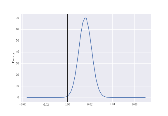
Now in order to compute \(p[p_R > p_B \rvert D_R, D_B]\) we can evaluate this as:
print ("Probability that button B gets MORE sign-ups than site B: %0.3f" % (delta_distribution >0).mean())
print ("Probability that button B gets LESS sign-ups than site B: %0.3f" % (delta_distribution < 0).mean())
which gives a \(99.8\%\) chance that blue is better, or a \(0.2\%\) chance that red is better.
Something more analytical.
What can we say in the limit as the number of observations tends to infinity? Let’s make a simplifying assumption that \(N_R= 2M_R\), \(k_R = M_R\) and \(N_B = 2M_B\), \(k_B = M_B\). Thus we should expect that we can show that the red and blue buttons are the same in the limit as \(M_R\) and \(M_B\) tend to \(+\infty\).
Let’s start by computing the expectation and varaince of the random variable \(p_R - p_B\):
\[\mathbb{E}(p_R - p_B \rvert D_R, D_B) = \mathbb{E}(p_R \rvert D_R) - \mathbb{E}(p_B \rvert D_B)\]with
\[\mathbb{E}(p_R \rvert D_R) = \frac{\int_0^1 \int_0^1 p_R^{M_R+1}(1-p_R)^{M_R} p_B^{M_B}(1-p_B)^{M_B}dp_R dp_B}{\int_0 ^1 \int_0^1p_R^{M_R}(1-p_R)^{M_R} p_B^{M_B}(1-p_B)^{M_B}dp_R dp_B } = \frac{B(M_R+2,M_R+1)}{B(M_R+1,M_R+1)}.\]We first do the computations for \(p_R\) and observe that the computations for \(p_B\) are identitical.
First, using the identity \(\frac{B(m+1,n)}{B(m,n)} = \frac{m B(m,n)}{m+n}\) we obtain
\[\mathbb{E}(p_R \rvert D_R) = \frac{M_R+1}{2M_R+3},\]and similarly,
\[\mathbb{E}(p_B \rvert D_B ) = \frac{M_B+1}{2M_B+3}.\]By definition:
\[\textrm{Var}(p_R) = \frac{1}{B(M_R+1,M_R+1)} \int_0^1 \left(p- \frac{n+1}{2n+3}\right)^2 p^n (1-p)^n dp\]Evaluating the above, we obtain:
\[\frac{B(M_R+3,M_R+1) - B(M_R+2,M_R+1)\frac{(M_R+1)}{(2M_R+3)} + \frac{(M_R+1)^2}{(2M_R+3)^2} B(M_R+1,M_R+1)}{B(M_R+1,M_R+1)}.\]Using the identity \(B(m+1,n) = \frac{mB(m,n)}{m+n}\) repeatedly and using the fact that \(M_R,M_B \to + \infty\), we have
\[\textrm{Var}(p_{R,B}) = o(1) \textrm{ as } M_R,M_B\to +\infty.\] \[\mathbb{E}(p_{R,B}) = \frac{1}{2} + o(1) \textrm{ as } M_R,M_B \to +\infty.\]Let \(f \in C^2([0,1])\), and let’s do a Taylor expansion of \(f\) around \(1/2\).
\[f(p) = f\left(0\right)+ f'\left(0)\right)p + \frac{1}{2}f''(\xi)p^2,\]where \(\xi \in [0,1/2]\).
Then we have
\[\int f(p_R-p_B) dF((p_R,p_B) \rvert M_R,M_B)\]\(= f\left(0\right) + f'\left(0\right) \left(\mathbb{E}(p_R \rvert D_R ) - \mathbb{E}(p_B \rvert D_B )\right) + \frac{1}{2} f''(\xi)\left(\textrm{Var}(p_R \rvert M_R)+\textrm{Var}(p_B \rvert M_B)\right)\),
which courtesy of the above, tends to \(f(0)\) as \(M_R, M_B \to +\infty\). This is equivalent to saying that
\[p_A \rvert D_R - p_B \rvert D_B \to \delta(0)\]in the sense of distributions as \(N_R,N_B \to +\infty\).
When the buttons aren’t equal?
In this case, by following the above, it’s clear that
\[\left(\mathbb{E}(p_R \rvert D_R ) - \mathbb{E}(p_B \rvert D_B )\right) \to \alpha\]for some \(\alpha \neq 0\). Then we repeat the above argument by doing a Taylor expansion of \(f\) around \(\alpha\) to obtain
\(= f\left(\alpha\right) + f'\left(\alpha\right) \left(\mathbb{E}(p_R \rvert D_R ) - \mathbb{E}(p_B \rvert D_B ) - \alpha \right) + \frac{1}{2} f''(\xi)\left(\textrm{Var}(p_R \rvert M_R)+\textrm{Var}(p_B \rvert M_B)\right)\),
which allows us to concldue that
\[p_A \rvert D_R - p_B \rvert D_B \to \delta(\alpha).\]Conclusion
Ultimately I believe that it’s far more natural to evaluate \(P[p_R > p_B \rvert D_R,D_B]\) which corresponds to the Bayesian framework. The main criticism of the framework is the assumption of a prior - why should we believe your prior? How does the prior affect convergence rates. However, as shown in this post, in order to quanitfy convergence rates, we need to actually get bounds on \(p(1-p)\) away from \(0\), which is essentially assuming some “prior” on the data.
Next steps
- A true comoparison will be to evaluate the convergence rates to the ‘ground truth’ (ie. the dirac measure) as \(N_R\) and \(N_B\) tend to \(+\infty\). This will be the next blog post.