Recall that in the last post, our aim was, given \(y \in \mathbb{R}^n\) and our features \(X \in \mathbb{R}^{n \times k}\) to find \(\beta \in \mathbb{R}^k\) which minimized:
\[\min_{\beta} \frac{1}{N} \sum_{i=1}^N(y_i - \beta \cdot \mathbf x_i)^2.\]We will explore the idea of over fitting and model selection in this section and see the benefits and drawbacks of various methods of parameter penalizaiton.
Regularized Linear Regression
Let’s say that our data points satisfy the following:
\[\mathbf{y} = 10\mathbf{x_0} + \epsilon,\]where \(\epsilon \sim \mathcal{N}(0,1)\).
We have \(\mathbb{R}^k\) features, so we can actually solve:
\[\mathbf{X}_k \beta = \mathbf{y},\]for a unique \(\beta \in \mathbb{R}^k\) where \(\mathbf{X}_k\) is the first \(k\) rows of \(X\). But wait! Doesn’t that mean we can pick up not just \(y\), but the noise terms from \(\epsilon\) as well? Yes! This is actually why we need regularization in the first place. Even though we have a collection of \(k\) orthogonal features, if we have \(j < k\) variables which influence \(y\), then we can over solve the system. This all seems very abstract though, so let’s construct a concrete example.
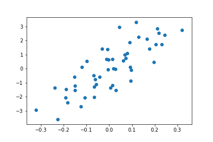
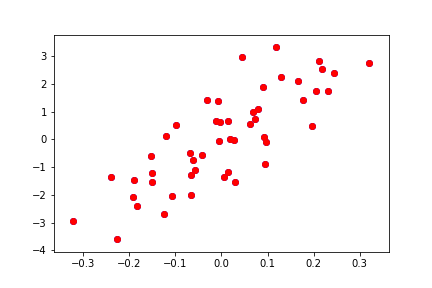
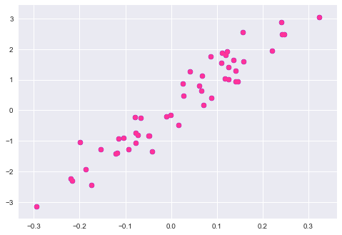
We are going to construct an orthogonal matrix of dimension \(50\) when \(y\) depends on only one variable:
\[\mathbf{y} = 10\mathbf{x_0} + \epsilon.\]What do you think will happen if we include only 1 feature? 20? 40? 80? Let’s write some code in Python to investigate. First let’s construct the orthogonal matrix and make a scatter plot to see how \(y\) depends on \(x\):
from scipy.stats import ortho_group
m = ortho_group.rvs(dim=50)
df_orth = pd.DataFrame(m).T


y = 10*x0 + np.random.normal(0, 1, 50)

plt.scatter(x0,y)
Now we have an orthogonal set of 50 features, but our output variable \(y\) depends on only one of them. What happens as we include more of the features into our model? If you followed the previous discussion, you should know the answer already.
from sklearn import datasets, linear_model

for d in range(0,80,20):
    regr = linear_model.LinearRegression(fit_intercept=False)
    X=df_orth.loc[:,0:d]
    # Train the model using the training sets
    regr.fit(X,y)

    # Make predictions using the testing set
    y_pred = regr.predict(X)
    plt.scatter(x0,y,color='b')
    plt.scatter(x0,y_pred,color='r')
    plt.show()
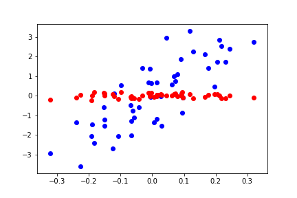
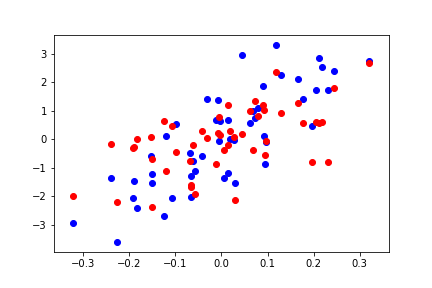
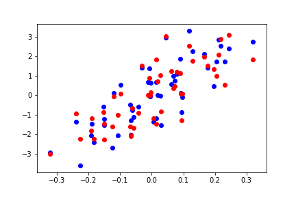
Do you see what’s going on here? As we increase the number of features, we are able to solve for every point exactly, which is not the true trend of the model.
Question: Why is this not ok? Isn’t that a perfect model?
Answer: No! This will not generalize properly to new data, as we will see when we evaluate these models using cross validation in this section.
First we define cross validation:
Cross Validation: Given features \(\mathbf X\) and output \(\mathbf y\), we train on a (ideally random) subset of rows of \(\mathbf X\) and \(\mathbf y\) which we will call \(\mathbf X_{\textrm{train}}\) and \(\mathbf y_{\textrm{train}}\) and evaluate the performance of the model on the remaining subsets which we call \(\mathbf X_{\textrm{test}}\) and \(\mathbf y_{\textrm{test}}\).
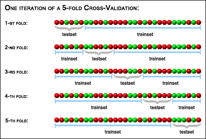
K-Fold Cross Validation: This is the standard method of evaluating models. It’s an extension of the above which involves splitting your data into \(K\) different folds, where you train on a random subset and evaluate on the remaining portion ofthe data set. The following picture explains this more clearly than words can.
Regularization - Penalizing the Size of Coefficients
In the example above, we see that as we increase the number of features we use, we over fit the model. But how do we quantify this and evaluate in a rigorous way? First we must discuss the notion of cross validation - evaluating your model on held out data.
First, let’s introduce the penalty term:
\[\sum_{k=1}^n (y_k- \beta \cdot \mathbf{x_k})^2 + \lambda \|\beta\|_{L^p}\]Equivalently, we can write the miniization problem as a maximum likelhihood problem:
\[\prod_{k=1}^N \frac{1}{2\sqrt{\pi}N} e^{-\frac{(y_k - \beta \cdot \mathbf{x_k})^2)}{\sigma^2} - \lambda \|\beta\|_{L^p}},\]which is just adding in a prior to our Gaussian.
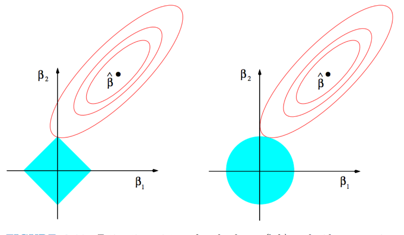
On the left in the figure above is the \(L^1\) norm and on the right the \(L^2\) norm. As a result of the square shape, \(L^1\) results in much sparser solutions (it’s more likely to hit a kink than a side), and \(L^2\) tends to spread out the error more. Before diving into this however, let’s consider for now the \(L^1\) norm and evaluate on held out data.
Now let’s try this on the data from before and see what we get. Note that this is a basic and crude example to demonstrate the method. The purpose is to show that our goal is to maximize our objective function over the possible parameters.
scores = []

alphas=[0,0.001,0.01]


for d in alphas:
    regr = linear_model.Lasso(alpha=d)
    X=df_orth

    # Train the model using the training sets
    regr.fit(X_train,y_train)

    # Make predictions using the testing set
    y_pred = regr.predict(X)
    scores.append(regr.score(X_test,y_test))
plt.plot(scores)
Let’s do this properly now using sklearn’s GridSearchCV package and 5-fold cross validation:
Lasso
# Set the parameters by cross-validation
from sklearn.grid_search import GridSearchCV

alphas=np.linspace(0.00001,1,1000)

model=linear_model.Lasso()
grid = GridSearchCV(estimator=model, param_grid=dict(alpha=alphas),cv=5)
grid.fit(X_train,y_train)

print(grid)
# summarize the results of the grid search
print(grid.best_score_)
print(grid.best_estimator_.alpha)
Output:
0.92
1e-5
Ridge
# Set the parameters by cross-validation
from sklearn.grid_search import GridSearchCV

alphas=np.linspace(1,1000,1000)

model=linear_model.Ridge()
grid = GridSearchCV(estimator=model, param_grid=dict(alpha=alphas),cv=5)
grid.fit(X_train,y_train)

print(grid)
# summarize the results of the grid search
print(grid.best_score_)
print(grid.best_estimator_.alpha)
Output:
-0.1678716256381307
53.0
Notice how Ridge performs much worse? (You can try other parameter ranges but you won’t see much of an improvement).
Question: Why do you think that Lasso is clearly out performing Ridge here?
Answer: Recall that Lasso is sparse so it will essentially remove all features except for \(\mathbf X[0]\), which is our true model! Ridge on the other hand, will spread the error throughout the features. Given that there are 49 useless features, that is enough noise to ruin any chance at a model.
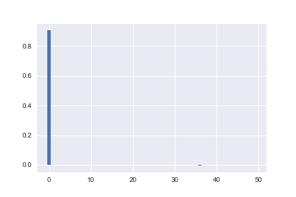
Let’s double check this. After training on Lasso, we have:
grid.best_estimator_.coef_Output:
array([ 0.90447066, -0. , 0. , 0. , 0. ,
-0. , -0. , 0. , 0. , -0. ,
0. , -0. , -0. , -0. , -0. ,
0. , 0. , -0. , -0. , 0. ,
-0. , -0. , -0. , -0. , 0. ,
0. , -0. , -0. , 0. , 0. ,
0. , 0. , -0. , 0. , -0. ,
0. , -0.00523794, -0. , -0. , -0. ,
-0. , 0. , -0. , 0. , 0. ,
-0. , 0. , -0. , -0. , 0. ])
Plotting these coefficients looks like:
For Ridge, we have:
grid.best_estimator_.coef_Output:
array([ 0.72697755, -0.07368477, 0.04537106, -0.00722343, 0.02094348,
-0.05251778, -0.12409298, 0.12192429, 0.10627641, 0.06119647,
0.13381586, -0.04695789, -0.05783079, -0.10238434, -0.09956115,
0.09799722, 0.11037942, -0.09609671, -0.0226349 , -0.10745485,
-0.03419379, 0.03693998, -0.02457642, -0.00328262, 0.00434185,
-0.01136398, 0.03571508, -0.06083133, -0.01302489, 0.10103576,
-0.01862894, 0.0104287 , -0.05681995, 0.05647496, -0.03031044,
0.02499557, -0.03367697, 0.03277902, 0.04771753, 0.17337222,
0.06181519, 0.03871668, 0.06484969, 0.00264665, 0.03209924,
0.01212371, 0.04856244, -0.10830154, -0.04072814, 0.05956078])
Plotting these coefficients looks like:

Notice how in the Lasso case, all of the coefficients are either zero, or two orders of magnitude smaller than \(X[0]\)? The eometric explanation above is the reason. For Ridge on the other hand, the coefficients spread the error out evenly as we expect.
A 3d interpretation to overfitting
Recall that we noted above that by adding enough dimensions, we can solve exactly the linear algebra problem:
\[\mathbf{X}_k \beta = \mathbf{y}.\]If we recall our scatter plot:
What we are really saying is that we have more flexibility if we add in other fake dimensions to our problem. Why is this? Essentially it boils down to now being able to use the hyperplane (instead of line) to hit the other points. To see this, let’s extend our scatter plot to include the variable \(\mathbf x_1\). We will then shift the plane so that it can hit the other points.
To understand this graph, it is crucial to realize that it does not matter where we assume the \(\mathbf x_2\) coordinate to lie here! We now have the added flexibility of finding a hyperplane that can hit any points. Let’s plot our original plane and a rotated one to illustrate:
from mpl_toolkits.mplot3d import axes3d
import matplotlib.pyplot as plt

for k in range(0,20,10):
    fig = plt.figure(figsize=(10,10))
    ax = plt.axes(projection='3d')

    ax.contour3D(X,Y,Z+k*Y, 50, cmap='binary')
    ax.scatter(xx, yy, z, color='#ff3399',s=40)

    ax.plot_wireframe(xx, xx.T, Z, rstride=5, cstride=5)

    #ax.plot(xx, yy, z, label='parametric curve')
    ax.set_xlabel('X_0')
    ax.set_ylabel('X_1')
    ax.set_zlabel('Y');


fig = plt.figure()
ax = fig.add_subplot(111, projection='3d')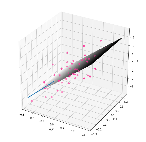
 As we can see, we can still hit all of our original points, but now we are able to rotate our plane to hit other points as well! The added dimension has given us flexibility, and this is why we can pick up additional variance.
Conclusion: Thus, Lasso is often better for feature selection. However once you have the “true” model, Ridge is better for performance according to most research (see papers of Andrew Ng if you are interested).